深度学习目录
目录
前言
该文是笔者关于优达学城无人驾驶工程师中深度学习部分的总结笔记,学习从头开始构建神经网络,使用TensorFlow和卷积神经网络,该部分实现了项目:Behavioral Cloning训练深度神经网络来自动驾驶汽车。
Lesson01:Neural Netowrks 神经网络
概要
Build and train neural networks from linear and logistic regression to backpropagation and multilayer perceptron networks.
构建和训练从线性回归和逻辑回归到反向传播和多层感知网络的神经网络。
01.神经网络 Neural Network
这些神经网络是基于数据训练的。本博客最后介绍如何在udacity模拟器中训练深度神经网络实现无人驾驶汽车, 首先,你将在模拟器中驾驶并记录参数,然后构建和训练一个从自己的驾驶方式中学习的神经网络,输入相机图像或传感器读数经过神经网络生成输出,汽车应该的转向角和纵向速度。
机器学习是人工智能的一个领域,它从数据中学习了解环境,而不是依赖人工设定规则。
深度学习是机器学习的一种方法,深度神经网络是描述大型多层神经网络的术语,感知器是神经网络的基本单元。
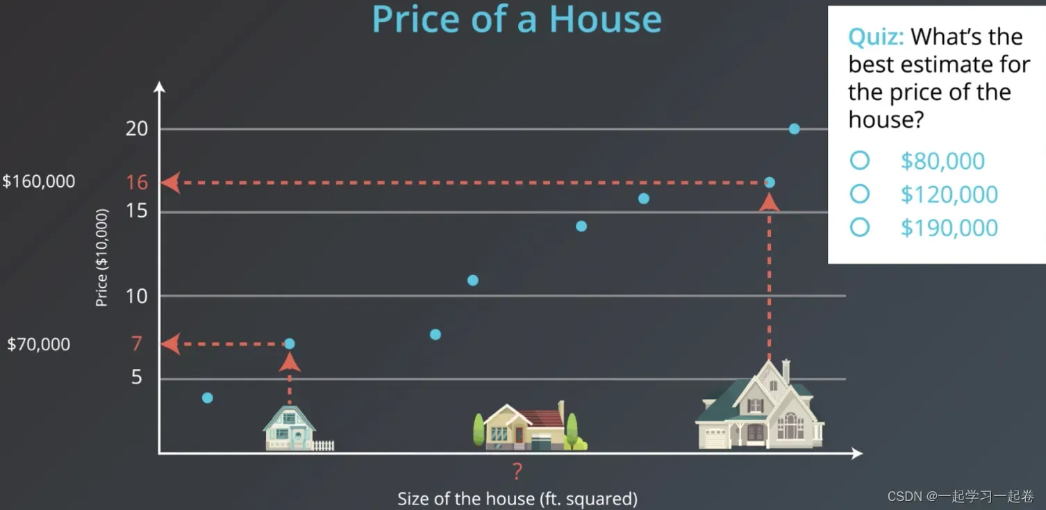
02.例子:房价
给定房子的面积来预测房子的价格,有一个价值70,000美元的小房子和一个价值160.000美元的大房子,想估计这些中型房子,那么应该怎么做呢?
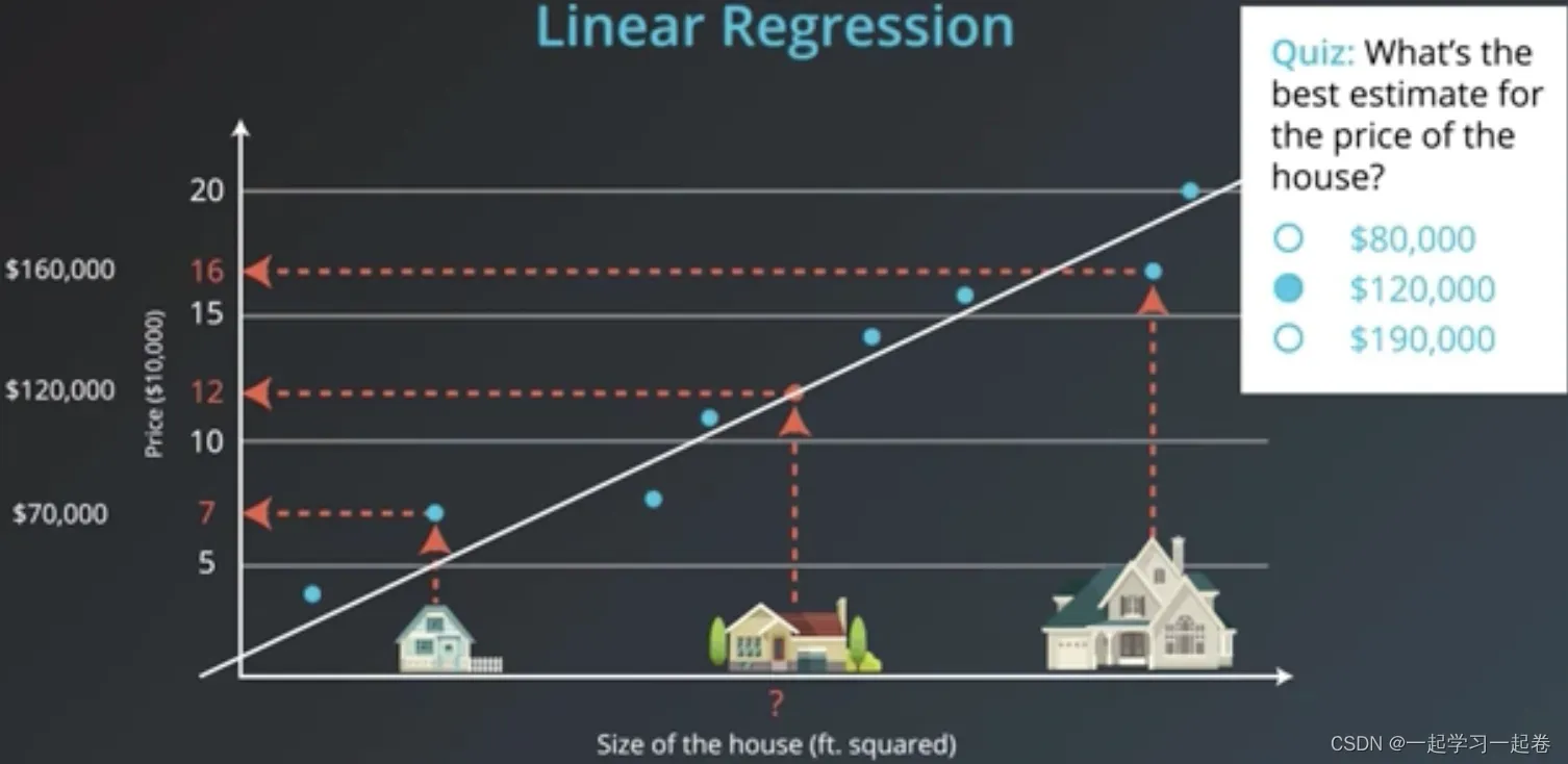
首先我们要先收集历史房价数据,将这些数据建立x为面积y为价格,如图这些蓝点是我们收集的数据,根据这些数据,你认为中型房屋价格的最佳估计是多少?
连接这些数据点找出最适合这些数据的线,即通过数据绘制最佳拟合线,这方法称为线性回归,
03.Classification Problem 分类问题
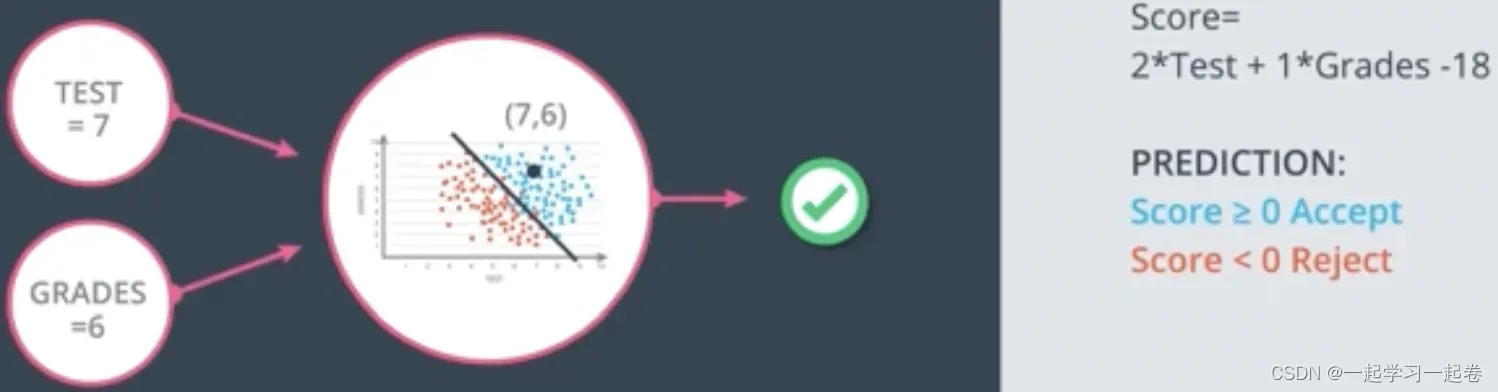
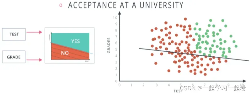
决定一位学生是否被录取,第一位学生Test=9 Grades=8被录取,第二位学生Test=3 Grades=4不被录取,预测第三位学生Test=7 Grades=6是否被录取?
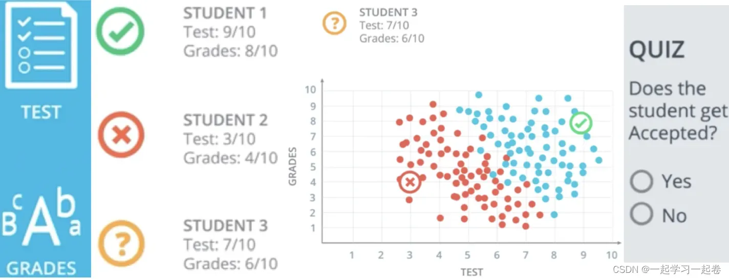
这个问题的第一个方法是在一个图表中绘制学生对应的分数为x,对应的等级为y。
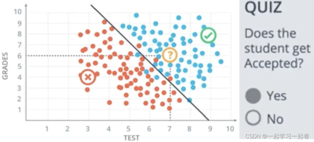
上面的表格被一条线很好地分隔开,这条线称为模型,这模型有几个错误,红点和蓝点没有被线完美分隔开,在线上方被录取,线下方被拒绝,那么应该如何找到这条线呢?
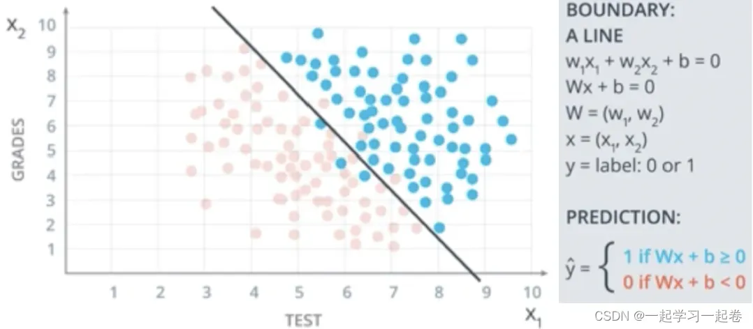
使用线性边界 Linear Boundaries
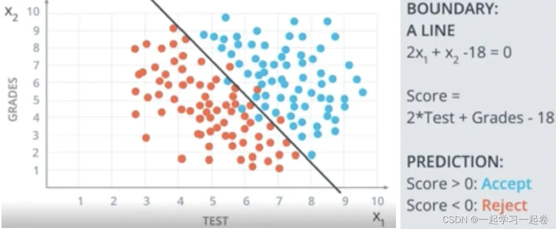
如图所示边界函数,简写为Wx+b=0
x为输入,w为权重,b为偏差,将标签值表示为Y,如果学生被录取Y=1,被拒绝Y=0,最后预测的结果是算法预测的标签,该算法的目标是让
Higher dimensions 更高维度

现在知道等级、测试、学生在班级中的排名,如何拟合这些三维数据呢?
x1表示等级,x2表示测试,x3表示班级排名,则方程不是在平面二维中的线,而是在三维空间中的平面。
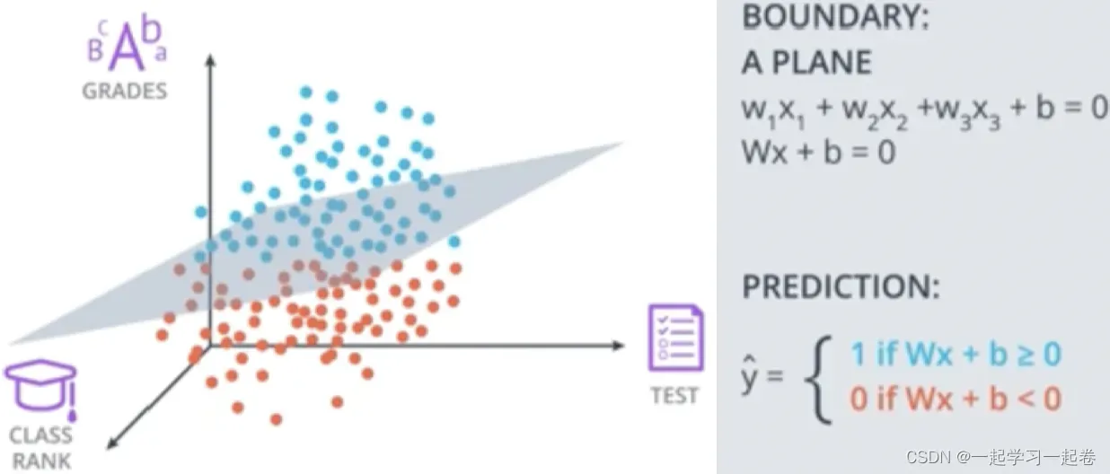
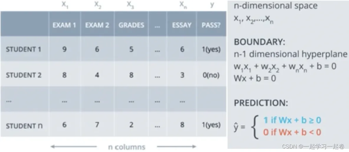
如上图所示,输入特征x,权重w,和满足 Wx+b 的偏差b的维度是多少?
W:(1 x n), x:(n x 1), b:(1 x 1)
04.Perceptrons 感知器
感知器是神经网络的构建块,将数据和边界线放在一个节点内,
增加输入x
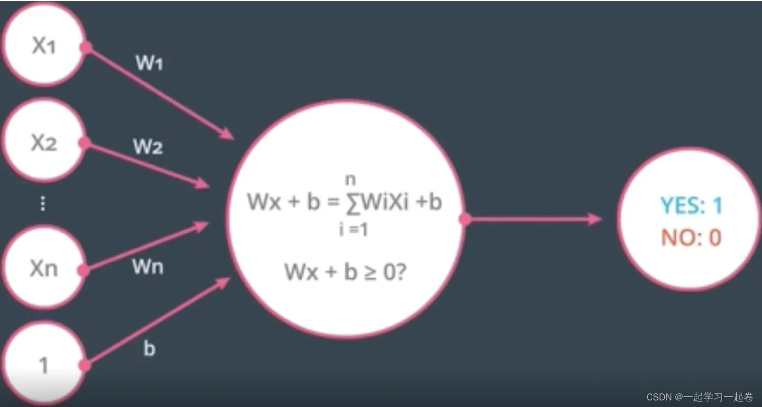
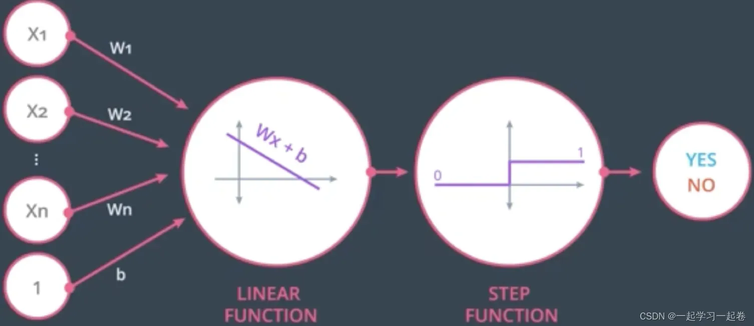
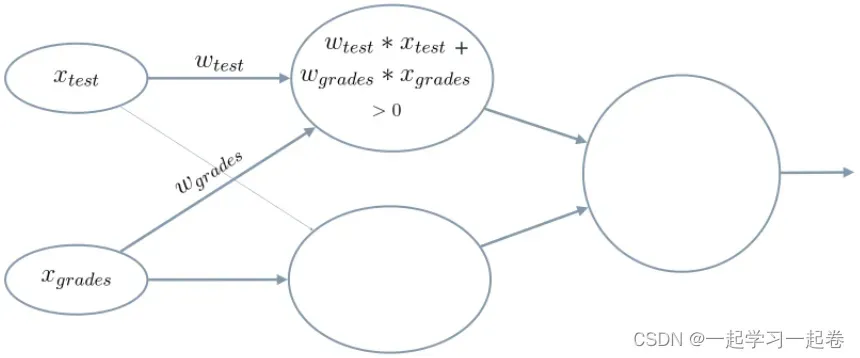
感知器可以看作节点的组合,第一个节点计算线性方程和权重的输入,第二个节点将阶跃函数应用于结果,
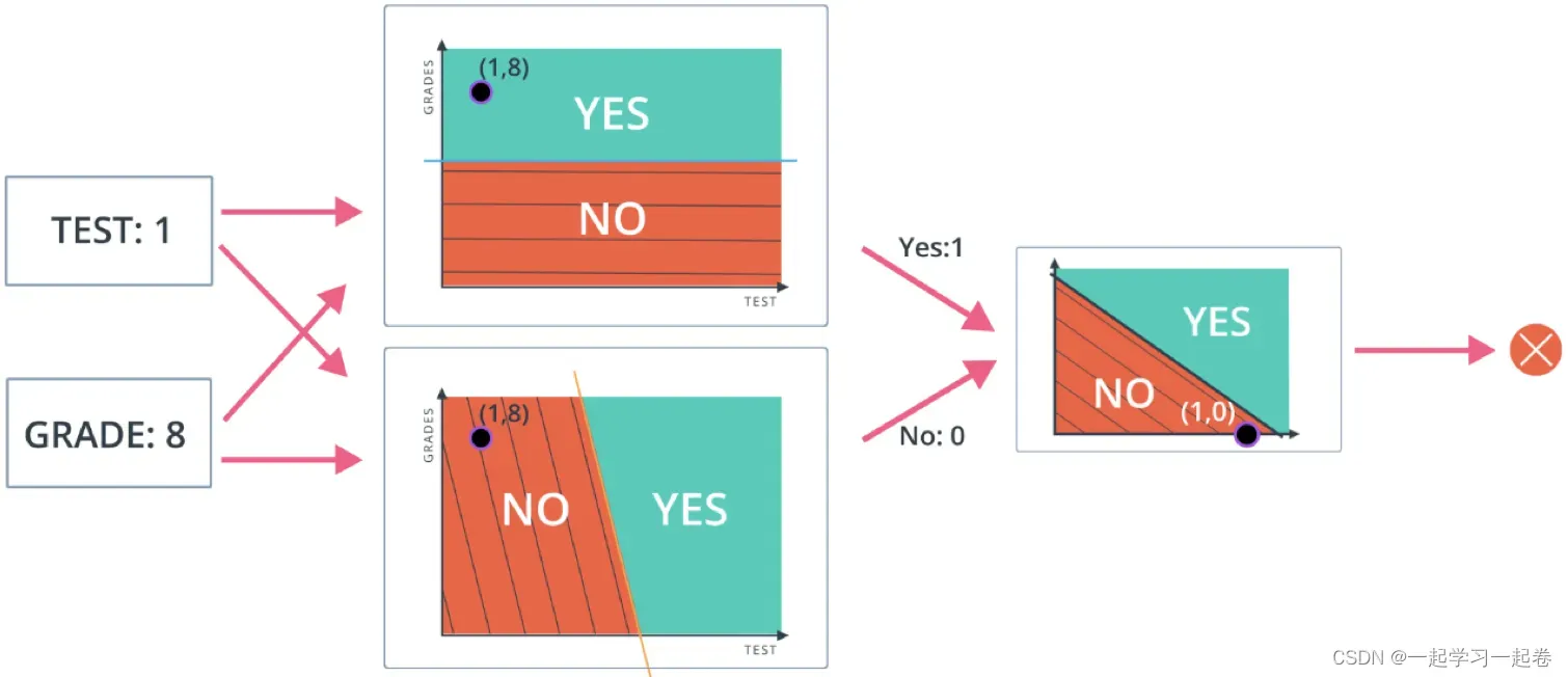
总结:现在已经了解简单的神经网络是如何做出决策,通过接收输入数据,计算处理该数据,最好输出结果,在上面的示例中,输入要么通过Test和Grades的阈值,要么不通过,因此两个类别是:是(通过阈值)和否(未通过阈值)。然后这些类别结合起来形成一个决定——例如,如果两个节点都产生“是”的输出,那么这个学生就会被大学录取。
这些单独的节点称为感知器或人工神经元,它们是神经网络的基本单元。
看看单个感知器如何处理输入数据, 当初始化一个神经网络时,不知道那些参数是对做出决定更重要,神经网络将使用反向传播来调整权重 weights,
将介绍权重,对输入数据求和,使用激活函数计算输出。
1.weights 权重
当输入x进入感知器时,它会乘以分配给该特定输入的权重值。例如,上面介绍的感知器有两个输入,分别为tests和grades,因此它有两个可以单独调整的权重。这些权重开始进行随机初始化,随着输入数据的计算与反向传播,网络会根据先前权重计算结果导致的错误分类来调整权重,这称为训练神经网络。
较高的权重意味着神经网络认为该输入比其他输入更重要,如果认为Test对大学录取没有任何影响,那么Test输入的权重将为零,并且不会影响感知器的输出。
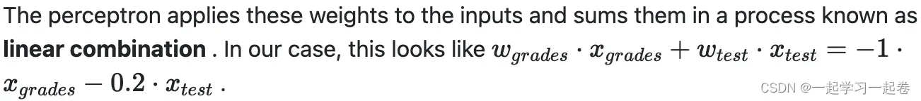
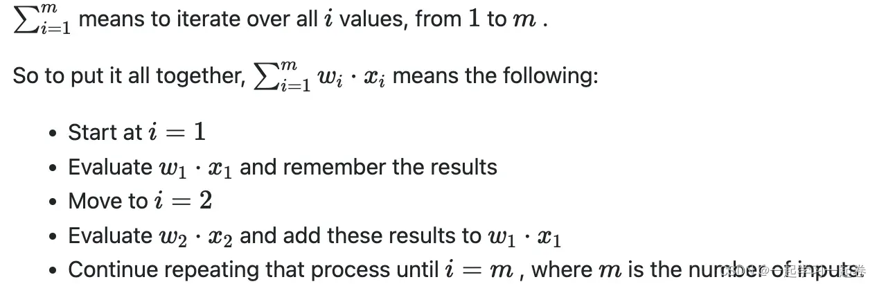
2.Summing the Input Data 对输入数据求和
将加权输入数据相加,即输入乘以权重然后全部相加,用于判断最终输出,

3.Calculating the Output with an Activation Function 使用激活函数计算输出
激活函数在给定节点输入的情况下决定节点输出是什么的函数?
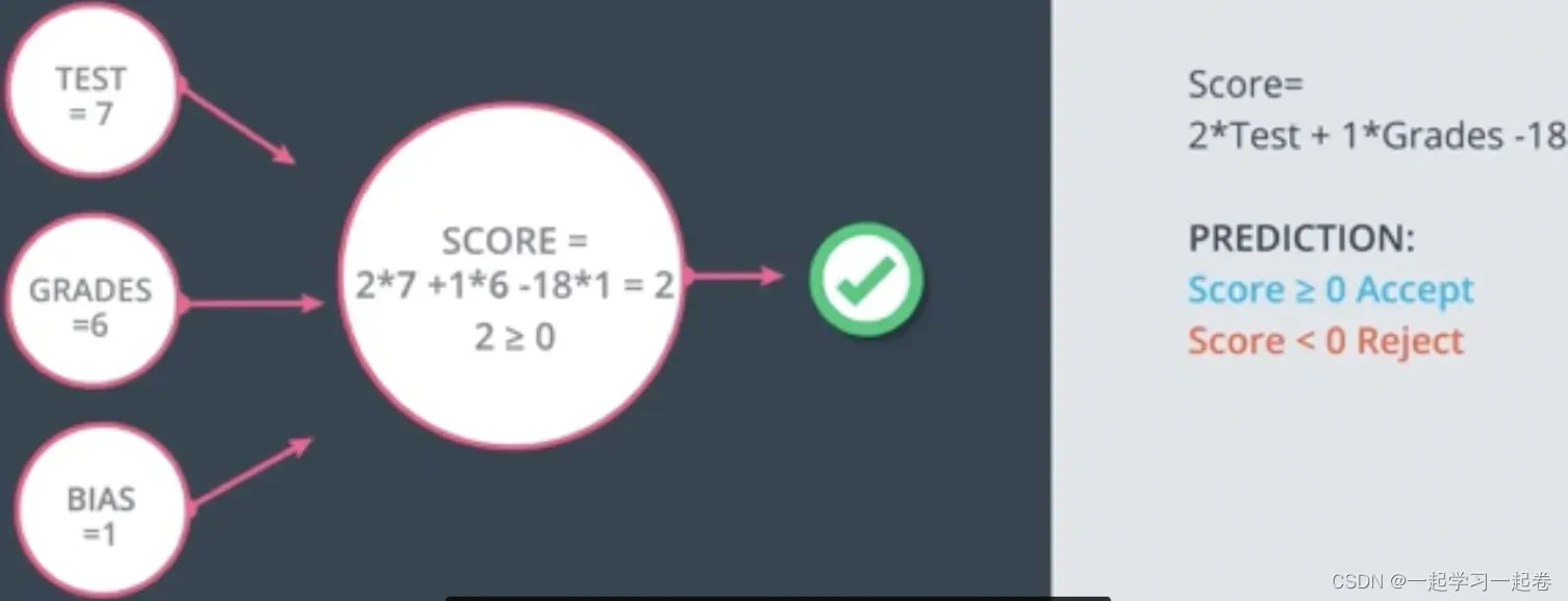
4.偏差 Bias
在线性组合的结果中添加一个值,称为偏差。如下图添加偏差 +3
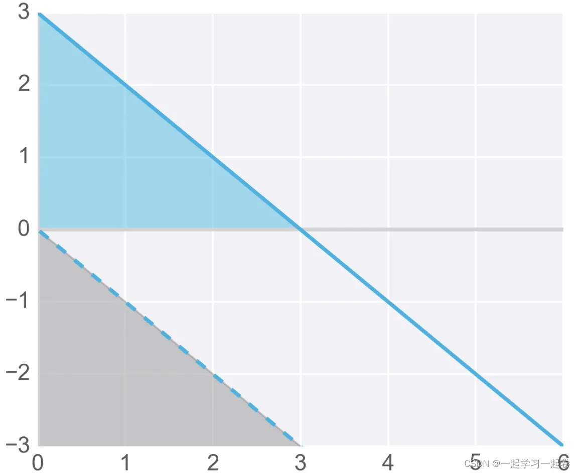
因为,开始不知道偏差的值,因此就像权重一样,偏差也可以在训练期间由神经网络更新和更改。所以在添加了一个偏差之后,我们现在有了一个完整的感知器公式:
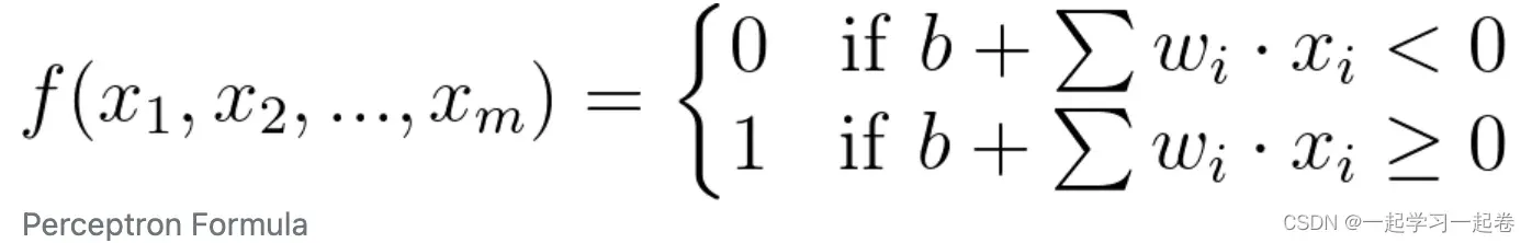
权重( wi) 和偏差 ( b ) 被分配一个随机值,然后使用梯度下降等学习算法对其进行更新。权重和偏差会发生变化,对下一个训练示例进行更准确的分类,并且神经网络“学习”数据中的模式。
05.Perceptron as Logical OPerators 感知器作为逻辑运算符
作为逻辑运算符,有常见的AND、OR和NOT运算符创建感知器,难以理解的XOR运算符创建感知器。
AND运算符接受两个输入并返回一个输出,输入可以是真或假,但是只有两个输入都为真时,输出才为真。如果变成一个感知器?第一步将表中的真值和假值变成一个1和0的表,然后绘制感知器由一条权重和偏差定义的线,有一个正区域为蓝色,负区域为红色。感知器就是划分每个点。
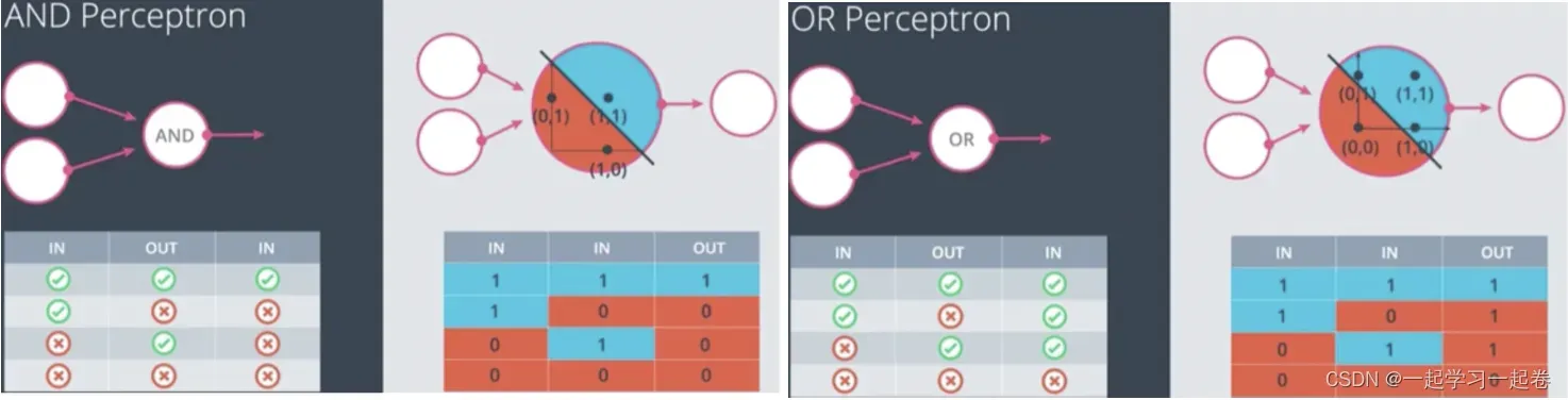
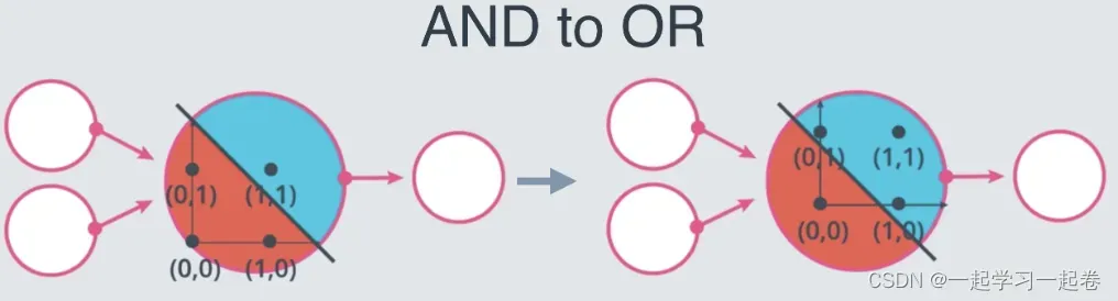
OR运算符,如果它的两个输入中任何一个为真,则输出真。
ADN代码实现
import pandas as pd
# TODO: Set weight1, weight2, and bias
weight1 = 0.0
weight2 = 0.0
bias = 0.0
# DON'T CHANGE ANYTHING BELOW
# Inputs and outputs
test_inputs = [(0, 0), (0, 1), (1, 0), (1, 1)]
correct_outputs = [False, False, False, True]
outputs = []
# Generate and check output
for test_input, correct_output in zip(test_inputs, correct_outputs):
    linear_combination = weight1 * test_input[0] + weight2 * test_input[1] + bias
    output = int(linear_combination >= 0)
    is_correct_string = 'Yes' if output == correct_output else 'No'
    outputs.append([test_input[0], test_input[1], linear_combination, output, is_correct_string])
# Print output
num_wrong = len([output[4] for output in outputs if output[4] == 'No'])
output_frame = pd.DataFrame(outputs, columns=['Input 1', '  Input 2', '  Linear Combination', '  Activation Output', '  Is Correct'])
if not num_wrong:
    print('Nice!  You got it all correct.\n')
else:
    print('You got {} wrong.  Keep trying!\n'.format(num_wrong))
print(output_frame.to_string(index=False))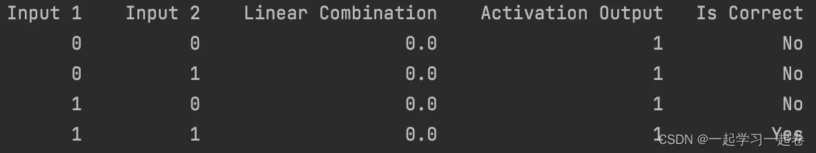
OR Perceptron Quiz
从 AND 感知器到 OR 感知器的两种方法是什么?
增加权重 Increase the weights
减少偏差的大小 Decrease the magnitude of the bias
NOT Perceptron
NOT感知器只有一个输入,当输入是0则输出1,当输入是1则输出0.
import pandas as pd
# TODO: Set weight1, weight2, and bias
weight1 = 0.0
weight2 = 0.0
bias = 0.0
# DON'T CHANGE ANYTHING BELOW
# Inputs and outputs
test_inputs = [(0, 0), (0, 1), (1, 0), (1, 1)]
correct_outputs = [True, False, True, False]
outputs = []

# Generate and check output
for test_input, correct_output in zip(test_inputs, correct_outputs):
    linear_combination = weight1 * test_input[0] + weight2 * test_input[1] + bias
    output = int(linear_combination >= 0)
    is_correct_string = 'Yes' if output == correct_output else 'No'
    outputs.append([test_input[0], test_input[1], linear_combination, output, is_correct_string])

# Print output
num_wrong = len([output[4] for output in outputs if output[4] == 'No'])
output_frame = pd.DataFrame(outputs, columns=['Input 1', '  Input 2', '  Linear Combination', '  Activation Output', '  Is Correct'])
if not num_wrong:
    print('Nice!  You got it all correct.\n')
else:
    print('You got {} wrong.  Keep trying!\n'.format(num_wrong))
print(output_frame.to_string(index=False))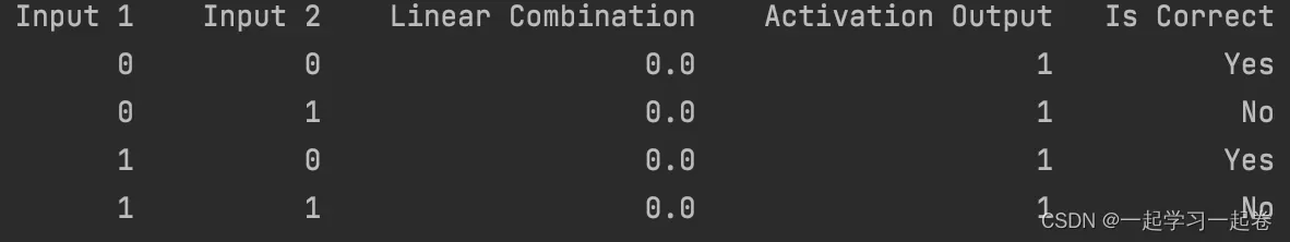
XOR Perceptron
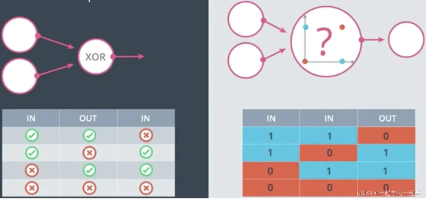
这四个点很难用一条线分开。
quiz:Build an XOR Multi-Layer perceptron 测验:构建 XOR 多层感知器
现在,让我们从 AND、NOT 和 OR 感知器构建一个多层感知器来创建 XOR 逻辑!
下面的神经网络包含 3 个感知器,A、B 和 C。最后一个 (AND) 已为您提供。神经网络的输入来自第一个节点。输出来自最后一个节点。下面的多层感知器计算 XOR。每个感知器都是 AND、OR 和 NOT 的逻辑运算。但是,感知器 A、B 和 C 并未指示它们的操作。在下面的测验中,为感知器设置正确的操作来计算 XOR。
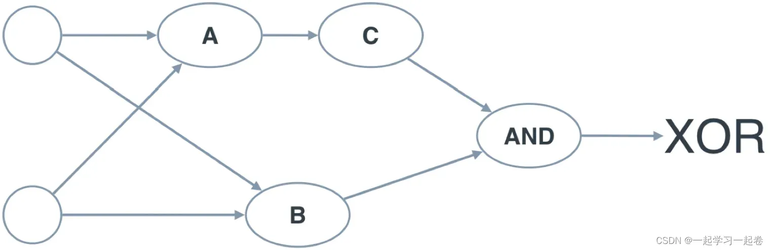
A:AND, B:OR, C:NOT
06.Perceptron Trick 感知器技巧
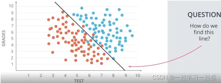
如何找到这条分隔线,How do we find this line?
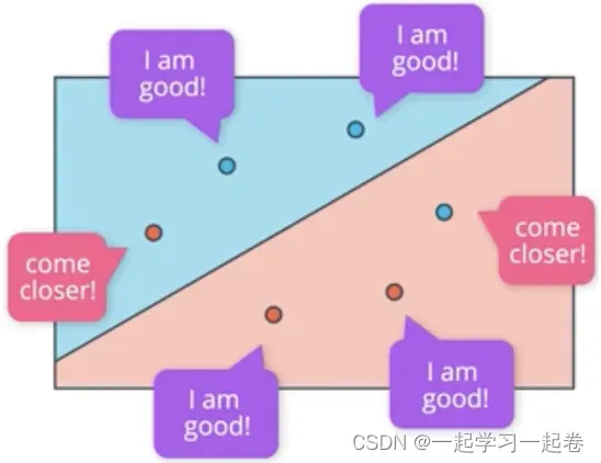
看一个例子带有三个蓝点和三个红点的小例子,通过选择一个随机线性方程从一个随机位置开始,这条线段将分别以蓝色和红色给出的正和负区域,

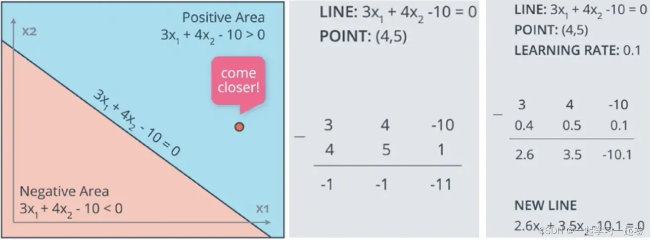
假设有线性方程 3×1 + 4×2 – 10 = 0,有一个错误点(4,5),那么如何让这个点更接近这条线呢?我们的方法是修改线的方程,使得线更靠近点,方程的参数是 3 4 -10,在这里给点(4,5)加个偏置单元1,从行的参数中减去这些数字,新行将具有参数-1 -1 -11,这条线将急剧接近点,但是我们不想太快的接近这个点,因为可能会不小心误分类了其他的点,希望线可以一小步点接近点,这就是学习率,乘以学习率以进行小步骤更新。
例如蓝色区域有点(1,1)为正区域点点,也被错误分类。
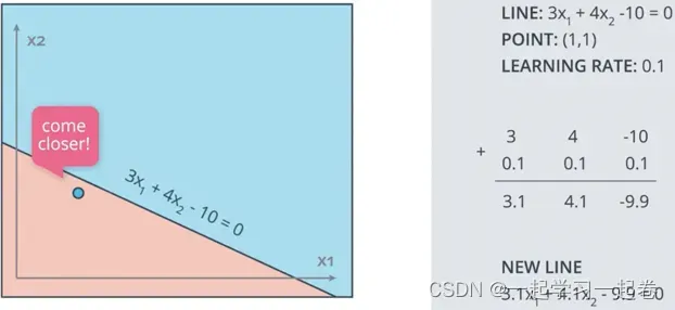
问题:对于第二个示例,线由 3×1 + 4×2 – 10 = 0 描述,如果学习率设置为 0.1,您必须应用感知器技巧多少次才能将线移动到(1, 1) 处的蓝点是否被正确分类?
07.Perceptron Algorithm 感知器算法
设计感知器算法,伪代码,用python对其进行编程。
编写这个感知器算法的伪代码。
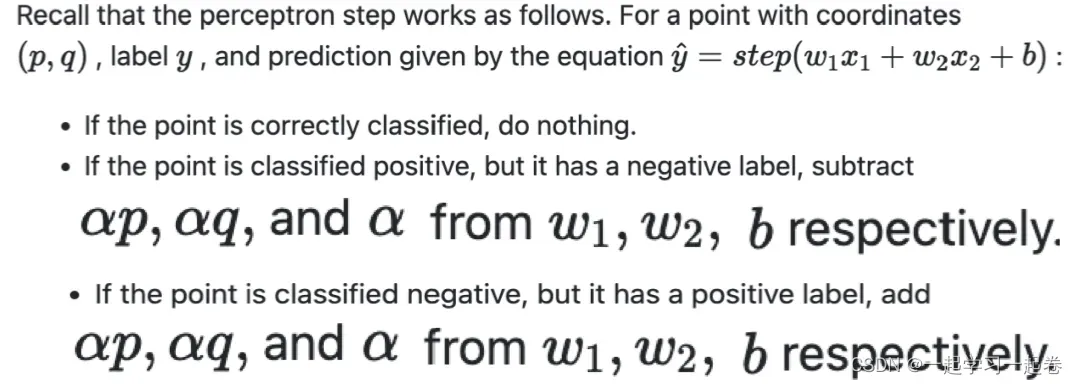
从随机权重开始,对于坐标x1到xn的每个错误分类点,执行以下操作,如果预测为零,这意味着该点是负区域中的正点,
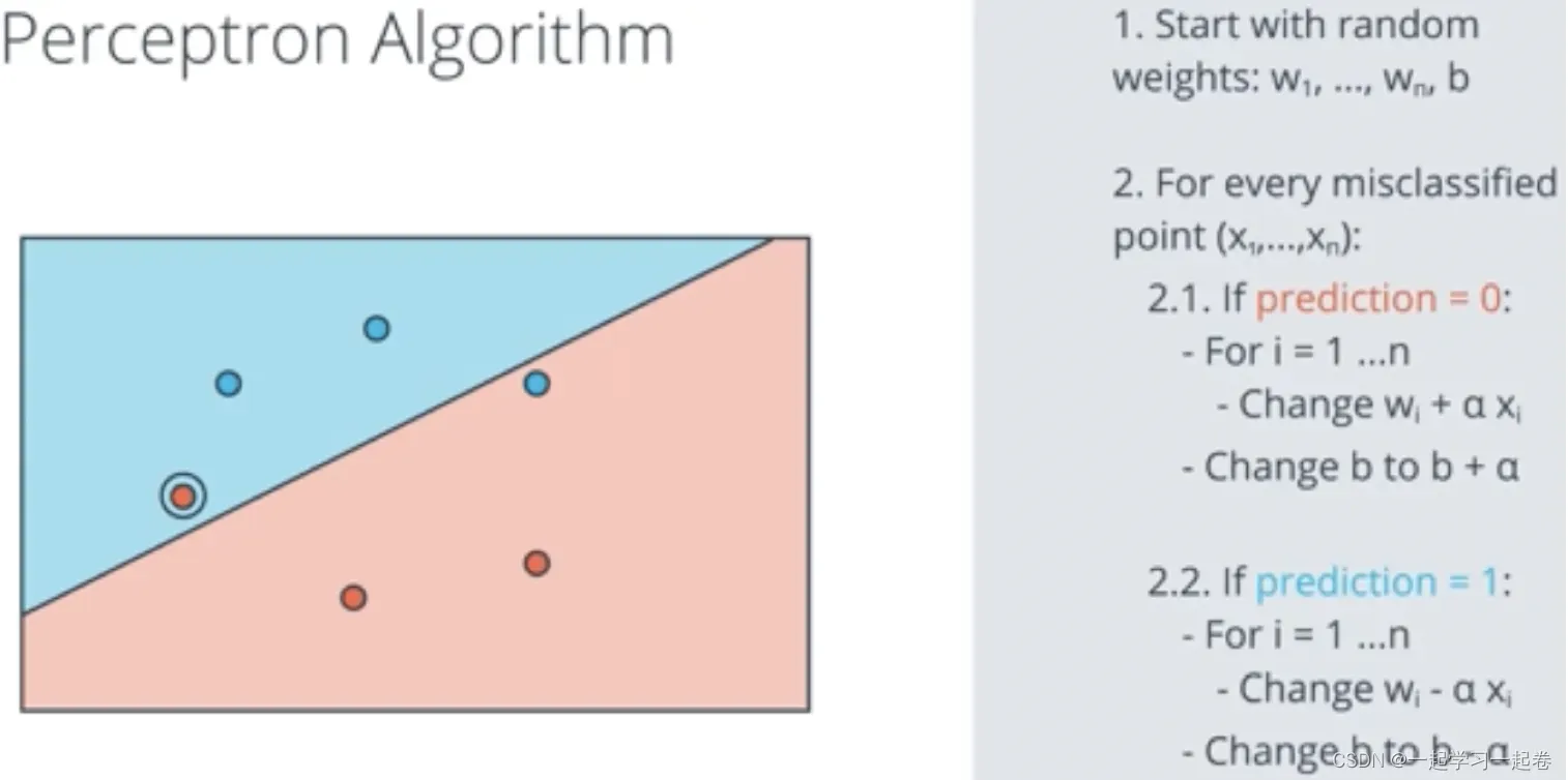
There’s a small error in the above video in that Wi should be updated to Wi=Wi+αxi (plus or minus depending on the situation).
Coding the Perceptron Algorithm 编码感知器算法
在这个测验中,您将有机会实现感知器算法来分离以下数据(在文件 data.csv 中给出)。
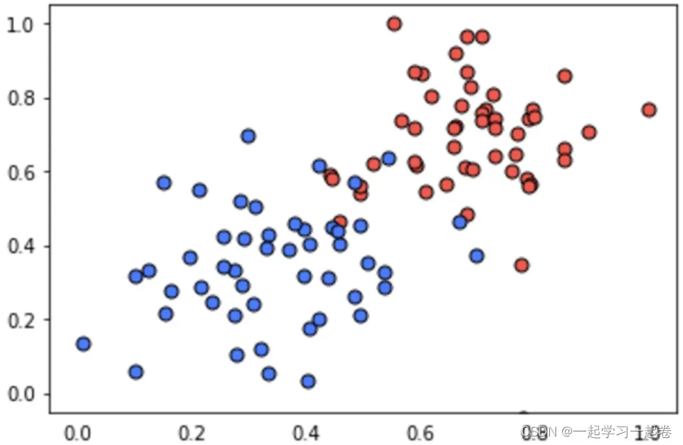
Perceptron.py代码
import numpy as np
# Setting the random seed, feel free to change it and see different solutions.
np.random.seed(42)

def stepFunction(t):
    if t >= 0:
        return 1
    return 0

def prediction(X, W, b):
    return stepFunction((np.matmul(X,W)+b)[0])

# TODO: Fill in the code below to implement the perceptron trick.
# The function should receive as inputs the data X, the labels y,
# the weights W (as an array), and the bias b,
# update the weights and bias W, b, according to the perceptron algorithm,
# and return W and b.
def perceptronStep(X, y, W, b, learn_rate = 0.01):
    # Fill in code
    return W, b

# This function runs the perceptron algorithm repeatedly on the dataset,
# and returns a few of the boundary lines obtained in the iterations,
# for plotting purposes.
# Feel free to play with the learning rate and the num_epochs,
# and see your results plotted below.
def trainPerceptronAlgorithm(X, y, learn_rate = 0.01, num_epochs = 25):
    x_min, x_max = min(X.T[0]), max(X.T[0])
    y_min, y_max = min(X.T[1]), max(X.T[1])
    W = np.array(np.random.rand(2,1))
    b = np.random.rand(1)[0] + x_max
    # These are the solution lines that get plotted below.
    boundary_lines = []
    for i in range(num_epochs):
        # In each epoch, we apply the perceptron step.
        W, b = perceptronStep(X, y, W, b, learn_rate)
        boundary_lines.append((-W[0]/W[1], -b/W[1]))
    return boundary_lines
solution.py代码
def perceptronStep(X, y, W, b, learn_rate = 0.01):
    for i in range(len(X)):
        y_hat = prediction(X[i],W,b)
        if y[i]-y_hat == 1:
            W[0] += X[i][0]*learn_rate
            W[1] += X[i][1]*learn_rate
            b += learn_rate
        elif y[i]-y_hat == -1:
            W[0] -= X[i][0]*learn_rate
            W[1] -= X[i][1]*learn_rate
            b -= learn_rate
    return W, b
data.csv 数据点
0.78051,-0.063669,1
0.28774,0.29139,1
0.40714,0.17878,1
0.2923,0.4217,1
0.50922,0.35256,1
0.27785,0.10802,1
0.27527,0.33223,1
0.43999,0.31245,1
0.33557,0.42984,1
0.23448,0.24986,1
0.0084492,0.13658,1
0.12419,0.33595,1
0.25644,0.42624,1
0.4591,0.40426,1
0.44547,0.45117,1
0.42218,0.20118,1
0.49563,0.21445,1
0.30848,0.24306,1
0.39707,0.44438,1
0.32945,0.39217,1
0.40739,0.40271,1
0.3106,0.50702,1
0.49638,0.45384,1
0.10073,0.32053,1
0.69907,0.37307,1
0.29767,0.69648,1
0.15099,0.57341,1
0.16427,0.27759,1
0.33259,0.055964,1
0.53741,0.28637,1
0.19503,0.36879,1
0.40278,0.035148,1
0.21296,0.55169,1
0.48447,0.56991,1
0.25476,0.34596,1
0.21726,0.28641,1
0.67078,0.46538,1
0.3815,0.4622,1
0.53838,0.32774,1
0.4849,0.26071,1
0.37095,0.38809,1
0.54527,0.63911,1
0.32149,0.12007,1
0.42216,0.61666,1
0.10194,0.060408,1
0.15254,0.2168,1
0.45558,0.43769,1
0.28488,0.52142,1
0.27633,0.21264,1
0.39748,0.31902,1
0.5533,1,0
0.44274,0.59205,0
0.85176,0.6612,0
0.60436,0.86605,0
0.68243,0.48301,0
1,0.76815,0
0.72989,0.8107,0
0.67377,0.77975,0
0.78761,0.58177,0
0.71442,0.7668,0
0.49379,0.54226,0
0.78974,0.74233,0
0.67905,0.60921,0
0.6642,0.72519,0
0.79396,0.56789,0
0.70758,0.76022,0
0.59421,0.61857,0
0.49364,0.56224,0
0.77707,0.35025,0
0.79785,0.76921,0
0.70876,0.96764,0
0.69176,0.60865,0
0.66408,0.92075,0
0.65973,0.66666,0
0.64574,0.56845,0
0.89639,0.7085,0
0.85476,0.63167,0
0.62091,0.80424,0
0.79057,0.56108,0
0.58935,0.71582,0
0.56846,0.7406,0
0.65912,0.71548,0
0.70938,0.74041,0
0.59154,0.62927,0
0.45829,0.4641,0
0.79982,0.74847,0
0.60974,0.54757,0
0.68127,0.86985,0
0.76694,0.64736,0
0.69048,0.83058,0
0.68122,0.96541,0
0.73229,0.64245,0
0.76145,0.60138,0
0.58985,0.86955,0
0.73145,0.74516,0
0.77029,0.7014,0
0.73156,0.71782,0
0.44556,0.57991,0
0.85275,0.85987,0
0.51912,0.62359,0
文章出处登录后可见!