softmax回归
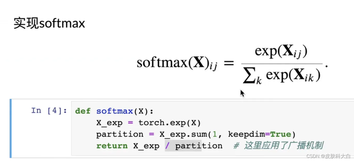
线性回归不同,softmax回归的输出单元从⼀个变成了多个,且引⼊了softmax运算使输出更适合离散值的预测和训练
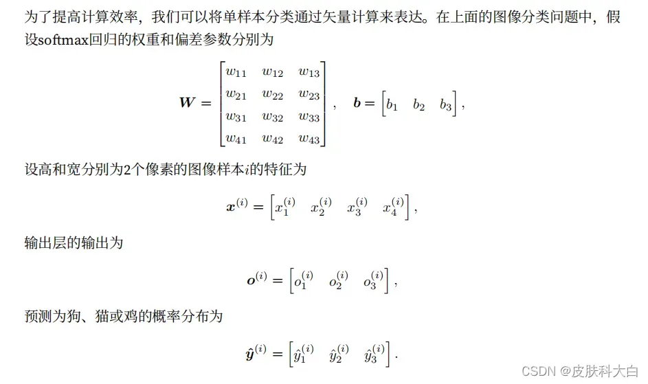
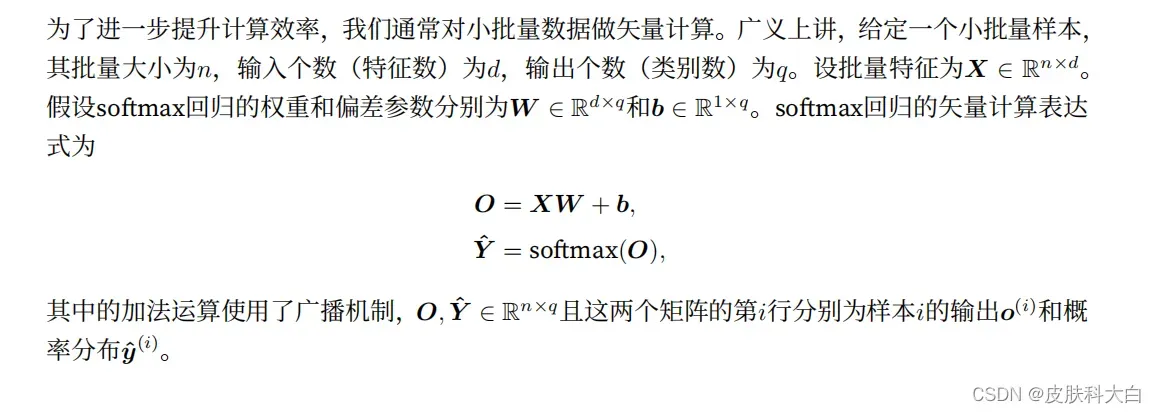
softmax回归跟线性回归⼀样将输⼊特征与权重做线性叠加。
它将logistic 激活函数推广到C类(C是神经网络模型的输出),而不仅仅是两类,是一种多分类器,如果C = 2,那么Softmax实际上变回了 logistic 回归。
与线性回归的⼀个主要不同在于,
softmax回归输入为向量
softmax回归的输出值个数等于标签⾥的类别数。
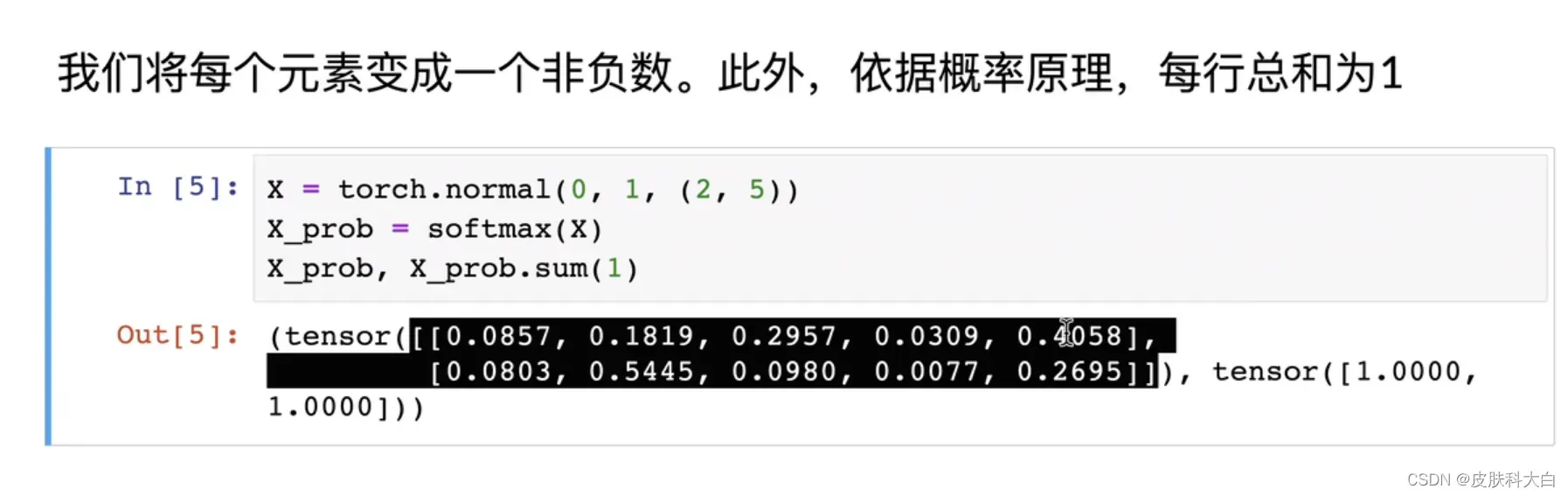
逻辑回归使用的是sigmoid函数,将w x + b \mathbf wx+bwx+b 的值映射到(0, 1)的区间,输出的结果为样本标签等于1的概率值;而softmax回归采用的是softmax函数,将w x + b \mathbf wx+bwx+b的值映射到[0, 1]的区间,输出的结果为一个向量,向量里的值为样本属于每个标签的概率值。


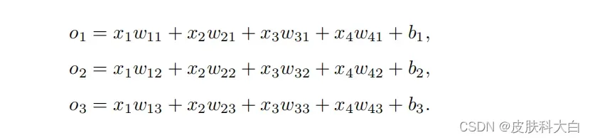
既然分类问题需要得到离散的预测输出,⼀个简单的办法是将输出值oi当作预测类别是i的置信度,并将值最⼤的输出所对应的类作为预测输出,即输出argmaxi oi。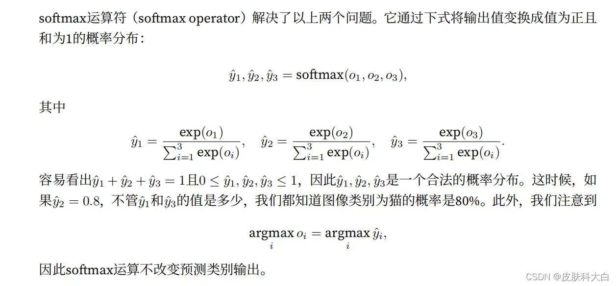
数据形状不变
y = torch.tensor([0, 2])
y_hat = torch.tensor([[0.1, 0.3, 0.6], [0.3, 0.2, 0.5]])
y_hat[[0, 1], y]
y_hat[[0, 1], y] 通过下标取值
先读取数据
输入为向量
import torch
from IPython import display
from d2l import torch as d2l

batch_size = 256
train_iter, test_iter = d2l.load_data_fashion_mnist(batch_size)
因为我们的数据集有10个类别,所以网络输出维度为10。 原始数据集中的每个样本都是(28 \times 28)的图像。 在本节中,我们将展平每个图像,把它们看作长度为784的向量。因此,权重将构成一个(784 \times 10)的矩阵, 偏置将构成一个(1 \times 10)的行向量。 与线性回归一样,我们将使用正态分布初始化我们的权重W,偏置初始化为0。
num_inputs = 784
num_outputs = 10

W = torch.normal(0, 0.01, size=(num_inputs, num_outputs), requires_grad=True)
b = torch.zeros(num_outputs, requires_grad=True)
定义模型
注意,将数据传递到模型之前,我们使用reshape函数将每张原始图像展平为向量。下面的代码定义了输入如何通过网络映射到输出
def net(X):
    return softmax(torch.matmul(X.reshape((-1, W.shape[0])), W) + b)
W.shape[0] 向量长度
-1 :batchsize
定义损失函数
def cross_entropy(y_hat, y):
    return - torch.log(y_hat[range(len(y_hat)), y])

cross_entropy(y_hat, y)
range(len(y_hat) :长度为len(y_hat)的向量
y_hat[range(len(y_hat)), y] :对应标号的预测值
y_hat :预测值,2*3
y: 真实值,长为2的向量
cross_entropy(y_hat, y) :长为2的向量
分类精度
当预测与标签分类y一致时,即是正确的。 分类精度即正确预测数量与总预测数量之比。虽然直接优化精度可能很困难(因为精度的计算不可导), 但精度通常是我们最关心的性能衡量标准,我们在训练分类器时几乎总会关注它。
如果y_hat是矩阵,那么假定第二个维度存储每个类的预测分数。 我们使用argmax获得每行中最大元素的索引来获得预测类别。 然后我们将预测类别与真实y元素进行比较。 由于等式运算符“==”对数据类型很敏感, 因此我们将y_hat的数据类型转换为与y的数据类型一致。 结果是一个包含0(错)和1(对)的张量。 最后,我们求和会得到正确预测的数量。
def accuracy(y_hat, y):  #@save
    """计算预测正确的数量"""
    if len(y_hat.shape) > 1 and y_hat.shape[1] > 1:
        y_hat = y_hat.argmax(axis=1)
    cmp = y_hat.type(y.dtype) == y
    return float(cmp.type(y.dtype).sum())
y_hat:预测值
y:真实值
y_hat.argmax(axis=1) :每一行中最大的值,预测分类的类别, 我们使用argmax获得每行中最大元素的索引来获得预测类别
y_hat.type(y.dtype):y_hat的数据类型转换为与y的数据类型一致
cmp.type(y.dtype):转换为与y的数据类型一致
cmp.type(y.dtype).sum():求和
float(cmp.type(y.dtype).sum()):转化为浮点数
accuracy(y_hat, y) / len(y)
类精度即正确预测数量与总预测数量之比
同样,对于任意数据迭代器data_iter可访问的数据集, 我们可以评估在任意模型net的精度。
def evaluate_accuracy(net, data_iter):  #@save
    """计算在指定数据集上模型的精度"""
    if isinstance(net, torch.nn.Module):
        net.eval()  # 将模型设置为评估模式,不计算梯度
    metric = Accumulator(2)  # 正确预测数、预测总数,累加器
    with torch.no_grad():
        for X, y in data_iter:
            metric.add(accuracy(net(X), y), y.numel())
    return metric[0] / metric[1]
net(X) :预测值
accuracy(net(X), y) 预测正确的样本数
y.numel():样本的总数
metric[0]:分类正确的样本数
metric[1]:总样本数
优化算法训练模型
def train_epoch_ch3(net, train_iter, loss, updater):  #@save
    """训练模型一个迭代周期(定义见第3章)"""
    # 将模型设置为训练模式
    if isinstance(net, torch.nn.Module):
        net.train()
    # 训练损失总和、训练准确度总和、样本数
    metric = Accumulator(3)
    for X, y in train_iter:
        # 计算梯度并更新参数
        y_hat = net(X)
        l = loss(y_hat, y)
        if isinstance(updater, torch.optim.Optimizer):
            # 使用PyTorch内置的优化器和损失函数
            updater.zero_grad()
            l.mean().backward()
            updater.step()
        else:
            # 使用定制的优化器和损失函数
            l.sum().backward()
            updater(X.shape[0])
        metric.add(float(l.sum()), accuracy(y_hat, y), y.numel())
    # 返回训练损失和训练精度
    return metric[0] / metric[2], metric[1] / metric[2]
class Animator:  #@save
    """在动画中绘制数据"""
    def __init__(self, xlabel=None, ylabel=None, legend=None, xlim=None,
                 ylim=None, xscale='linear', yscale='linear',
                 fmts=('-', 'm--', 'g-.', 'r:'), nrows=1, ncols=1,
                 figsize=(3.5, 2.5)):
        # 增量地绘制多条线
        if legend is None:
            legend = []
        d2l.use_svg_display()
        self.fig, self.axes = d2l.plt.subplots(nrows, ncols, figsize=figsize)
        if nrows * ncols == 1:
            self.axes = [self.axes, ]
        # 使用lambda函数捕获参数
        self.config_axes = lambda: d2l.set_axes(
            self.axes[0], xlabel, ylabel, xlim, ylim, xscale, yscale, legend)
        self.X, self.Y, self.fmts = None, None, fmts

    def add(self, x, y):
        # 向图表中添加多个数据点
        if not hasattr(y, "__len__"):
            y = [y]
        n = len(y)
        if not hasattr(x, "__len__"):
            x = [x] * n
        if not self.X:
            self.X = [[] for _ in range(n)]
        if not self.Y:
            self.Y = [[] for _ in range(n)]
        for i, (a, b) in enumerate(zip(x, y)):
            if a is not None and b is not None:
                self.X[i].append(a)
                self.Y[i].append(b)
        self.axes[0].cla()
        for x, y, fmt in zip(self.X, self.Y, self.fmts):
            self.axes[0].plot(x, y, fmt)
        self.config_axes()
        display.display(self.fig)
        display.clear_output(wait=True)
def train_ch3(net, train_iter, test_iter, loss, num_epochs, updater):  #@save
    """训练模型(定义见第3章)"""
    animator = Animator(xlabel='epoch', xlim=[1, num_epochs], ylim=[0.3, 0.9],
                        legend=['train loss', 'train acc', 'test acc'])
    for epoch in range(num_epochs):
        train_metrics = train_epoch_ch3(net, train_iter, loss, updater)
        test_acc = evaluate_accuracy(net, test_iter)
        animator.add(epoch + 1, train_metrics + (test_acc,))
    train_loss, train_acc = train_metrics
    assert train_loss < 0.5, train_loss
    assert train_acc <= 1 and train_acc > 0.7, train_acc
    assert test_acc <= 1 and test_acc > 0.7, test_acc
lr = 0.1

def updater(batch_size):
    return d2l.sgd([W, b], lr, batch_size)
num_epochs = 10
train_ch3(net, train_iter, test_iter, cross_entropy, num_epochs, updater)
Fashion-MNIST数据集, 并设置数据迭代器的批量大小为256。
import torch
from IPython import display
from d2l import torch as d2l

batch_size = 256
train_iter, test_iter = d2l.load_data_fashion_mnist(batch_size)
num_inputs = 784
num_outputs = 10

W = torch.normal(0, 0.01, size=(num_inputs, num_outputs), requires_grad=True)
b = torch.zeros(num_outputs, requires_grad=True)
def net(X):
    return softmax(torch.matmul(X.reshape((-1, W.shape[0])), W) + b)
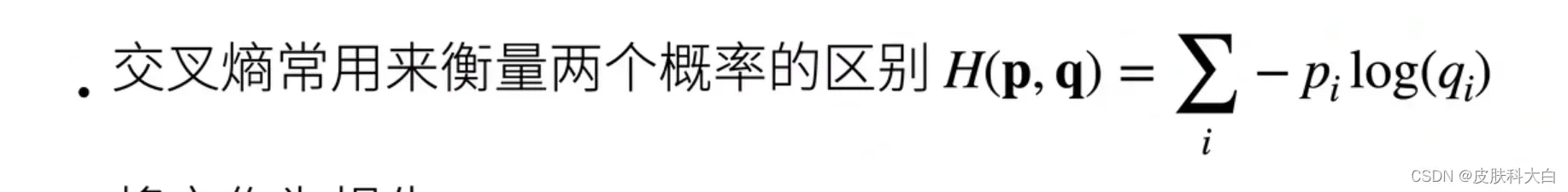
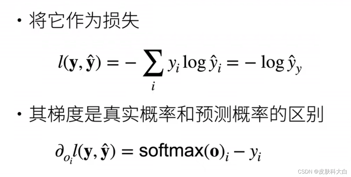
交叉熵采用真实标签的预测概率的负对数似然。
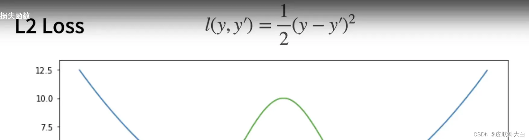
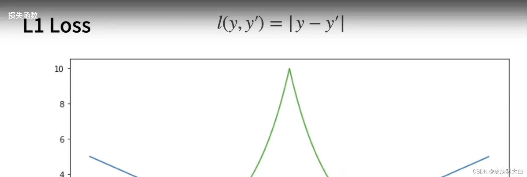
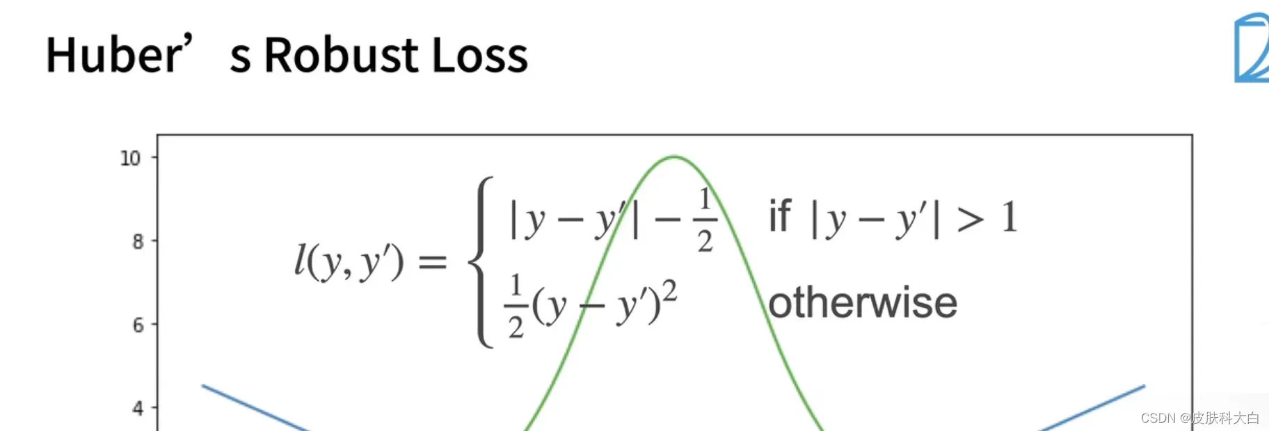
损失函数
文章出处登录后可见!