非线性回归
目标
- 区分线性回归和非线性回归
- 用py实现非线性回归
如果数据表现出一个曲线的趋势,那么相比于非线性回归,线性回归就不会产生一个非常精确的结果,因为线性回归假设数据是线性的。就让我们通过一个例子学习一下非线性回归。在这篇博客中我们对中国1960年到2014年的GDP拟合了一个非线性模型。
导入相关库
import numpy as np
import matplotlib.pyplot as plt
%matplotlib inline
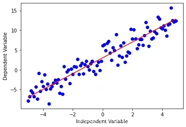
虽然线性回归在有的数据集上表现的很好,但是它不能应用到所有数据集。首先我们回想一下线性回归,它是拟合因变量y和自变量x,方程是很简单的,比如。
下面用代码来看看。
x = np.arange(-5.0, 5.0, 0.1)

##You can adjust the slope and intercept to verify the changes in the graph
y = 2*(x) + 3
y_noise = 2 * np.random.normal(size=x.size)
ydata = y + y_noise
#plt.figure(figsize=(8,6))
plt.plot(x, ydata,  'bo')
plt.plot(x,y, 'r')
plt.ylabel('Dependent Variable')
plt.xlabel('Independent Variable')
plt.show()
非线性回归是用一种拟合自变量 和因变量
之间的非线性关系的一种方法。
比如下面是一个多项式。
非线性函数有指数、对数、分数等元素
也可以是这种复杂的形式
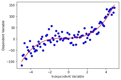
让我们看看这个三次函数
x = np.arange(-5.0, 5.0, 0.1)

##You can adjust the slope and intercept to verify the changes in the graph
y = 1*(x**3) + 1*(x**2) + 1*x + 3
# 加点噪音,也就是随机数
y_noise = 20 * np.random.normal(size=x.size)
ydata = y + y_noise
plt.plot(x, ydata,  'bo')
plt.plot(x,y, 'r')
plt.ylabel('Dependent Variable')
plt.xlabel('Independent Variable')
plt.show()
还有一些其他的形式
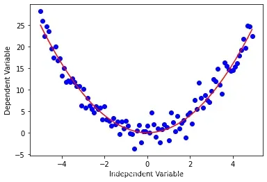
二次函数
x = np.arange(-5.0, 5.0, 0.1)

##You can adjust the slope and intercept to verify the changes in the graph

y = np.power(x,2)
y_noise = 2 * np.random.normal(size=x.size)
ydata = y + y_noise
plt.plot(x, ydata,  'bo')
plt.plot(x,y, 'r')
plt.ylabel('Dependent Variable')
plt.xlabel('Independent Variable')
plt.show()
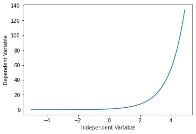
指数函数
X = np.arange(-5.0, 5.0, 0.1)

##You can adjust the slope and intercept to verify the changes in the graph

Y= np.exp(X)

plt.plot(X,Y)
plt.ylabel('Dependent Variable')
plt.xlabel('Independent Variable')
plt.show()
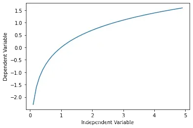
对数
X = np.arange(-5.0, 5.0, 0.1)

Y = np.log(X)

plt.plot(X,Y)
plt.ylabel('Dependent Variable')
plt.xlabel('Independent Variable')
plt.show()
Sigmoidal/Logistic
X = np.arange(-5.0, 5.0, 0.1)


Y = 1-4/(1+np.power(3, X-2))

plt.plot(X,Y)
plt.ylabel('Dependent Variable')
plt.xlabel('Independent Variable')
plt.show()

非线性回归的例子
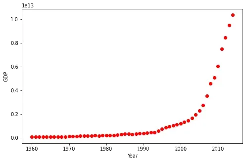
我们将要拟合中国从1960年到2014年的GDP数据。我们下载的数据有两列,第一列是年份,从1960到2014,第二列是对应年份的国内生产总值(美元)。
import numpy as np
import pandas as pd
df = pd.read_csv("china_gdp.csv")
df.head(10)
| Year | Value | |
|---|---|---|
| 0 | 1960 | 5.918412e+10 |
| 1 | 1961 | 4.955705e+10 |
| 2 | 1962 | 4.668518e+10 |
| 3 | 1963 | 5.009730e+10 |
| 4 | 1964 | 5.906225e+10 |
| 5 | 1965 | 6.970915e+10 |
| 6 | 1966 | 7.587943e+10 |
| 7 | 1967 | 7.205703e+10 |
| 8 | 1968 | 6.999350e+10 |
| 9 | 1969 | 7.871882e+10 |
数据可视化
数据有点像logistic或者指数函数,一开始增长得特别慢,从2005年开始,增长速度就非常显著了,在2010年代略微减速。
plt.figure(figsize=(8,5))
x_data, y_data = (df["Year"].values, df["Value"].values)
plt.plot(x_data, y_data, 'ro')
# plt.stem(x_data, y_data)
plt.ylabel('GDP')
plt.xlabel('Year')
plt.show()
选择模型
从第一眼看这个散点图,我就感觉logistic函数会不错,因为一开始增长很慢、中间增长很快、最后又慢了下来
就像下面这样:
X = np.arange(-5.0, 5.0, 0.1)
Y = 1.0 / (1.0 + np.exp(-X))

plt.plot(X,Y)
plt.ylabel('Dependent Variable')
plt.xlabel('Independent Variable')
plt.show()
![[外链图片转存失败,源站可能有防盗链机制,建议将图片保存下来直接上传(img-7EHjyekz-1655197597832)(output_28_0.png)]](https://aitechtogether.com/wp-content/uploads/2022/06/642fd00f-d066-4ec1-a3c9-d4f9a4af60b0.webp)
logsitic函数的方程如下
: 控制曲线的陡度,
: x轴上平移
构建模型
现在,让我们构建我们的回归模型并且初始化参数
def sigmoid(x, Beta_1, Beta_2):
     y = 1 / (1 + np.exp(-Beta_1*(x-Beta_2)))
     return y
首先随便搞两个参数
beta_1 = 0.10
beta_2 = 1990.0

#logistic function
Y_pred = sigmoid(x_data, beta_1 , beta_2)

#plot initial prediction against datapoints
plt.plot(x_data, Y_pred*15000000000000.)
plt.plot(x_data, y_data, 'ro')
![[外链图片转存失败,源站可能有防盗链机制,建议将图片保存下来直接上传(img-fdiZTFbv-1655197597833)(output_33_1.png)]](https://aitechtogether.com/wp-content/uploads/2022/06/1df819af-ae79-4ffa-a317-17bd9ad8a0ae.webp)
我们的目标是找到最好的参数。
第一步把x和y都标准化一下。
# Lets normalize our data
xdata =x_data/max(x_data)
ydata =y_data/max(y_data)
如何找到拟合曲线最好的参数?
我们可以使用curve_fit,它使用非线性最小二乘来拟合我们的sigmoid函数。 优化参数值,使sigmoid(xdata, *popt) – ydata的残差平方和最小化。
Popt是我们的优化参数。
from scipy.optimize import curve_fit
popt, pcov = curve_fit(sigmoid, xdata, ydata)
#print the final parameters
print(" beta_1 = %f, beta_2 = %f" % (popt[0], popt[1]))
beta_1 = 690.451711, beta_2 = 0.997207
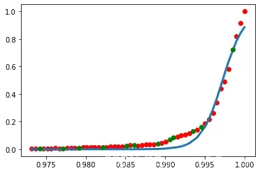
现在画一下我们的回归模型。
x = np.linspace(1960, 2015, 55)
x = x/max(x)
plt.figure(figsize=(8,5))
y = sigmoid(x, *popt)
plt.plot(xdata, ydata, 'ro', label='data')
plt.plot(x,y, linewidth=3.0, label='fit')
plt.legend(loc='best')
plt.ylabel('GDP')
plt.xlabel('Year')
plt.show()
![[外链图片转存失败,源站可能有防盗链机制,建议将图片保存下来直接上传(img-PIAwrPIA-1655197597833)(output_39_0.png)]](https://aitechtogether.com/wp-content/uploads/2022/06/114cff1a-4f16-4de8-9f85-215275fa3807.webp)
评估模型
虽然看上去不错,但是在运行过程中有时竟是负的,而且就是
很大的时候在测试集上实际效果也不是很好,所以还是不很靠谱。
# 把数据分为训练集和测试集
msk=np.random.rand(len(df))<0.8
# print(msk)
train_x=xdata[msk]
test_x=xdata[~msk]
train_y=ydata[msk]
test_y=ydata[~msk]

# 用训练集建立一个模型
popt,pcov=curve_fit(sigmoid,train_x,train_y)

yyy = sigmoid(train_x, *popt)
plt.plot(train_x, train_y, 'ro', label='data')
plt.plot(train_x,yyy, linewidth=3.0, label='fit')
plt.plot(test_x, test_y, 'go', label='data')
# 在测试集上预测
y_hat=sigmoid(test_x,*popt)
print("test_x:",test_x*sum(df["Year"]))
print("test_y:",test_y*sum(df['Value']))
print("y_hat:",y_hat*sum(df['Value']))
# 评估
print("Mean absolute error: %.2f" % np.mean(np.absolute(y_hat - test_y)))
print("Residual sum of squares (MSE): %.2f" % np.mean((y_hat - test_y) ** 2))
from sklearn.metrics import r2_score
print("R2-score: %.2f" % r2_score(test_y,y_hat) )
test_x: [106463.34160874 106788.91757696 107005.96822244 107331.54419067
 107657.12015889 107765.64548163 108091.22144985 108254.00943396
 108308.27209533 108579.58540218 108688.11072493 109122.21201589]
test_y: [3.56342870e+11 5.34252726e+11 8.56103610e+11 1.13258445e+12
 1.96991285e+12 2.28075199e+12 3.24347532e+12 5.58752067e+12
 6.57072900e+12 1.01688021e+13 1.25937257e+13 5.71889161e+13]
y_hat: [3.13221434e+06 2.82948697e+07 1.22728310e+08 1.10865316e+09
 1.00138972e+10 2.08527024e+10 1.87974610e+11 5.62290529e+11
 8.08915481e+11 4.80484704e+12 9.38891854e+12 5.66862461e+13]
Mean absolute error: 0.03
Residual sum of squares (MSE): 0.00
R2-score: 0.96
文章出处登录后可见!