目录
Yolov5 目标检测

一、工程目录及所需的配置文件解析
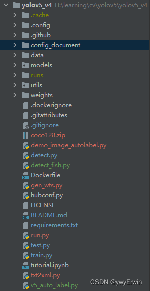
整个目录结构如下图所示:
其中config_document包含yolov5的预训练模型和模型参数等的配置文件,结构如下图所示:
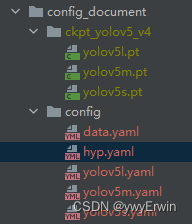
其中ckpt_yolov5_v4文件夹为yolov5的预训练模型,其为基于coco数据集共80个类别,已经训练好的初始模型参数,在数据量较少的情况下使用预训练模型可使训练过程较快速收敛(迁移学习),因为预训练模型已经有80个类别相对较好的权重和偏差,相比从头训练,模型权重为0或0-1间随机选取,效果更好,更易收敛。
配置文件
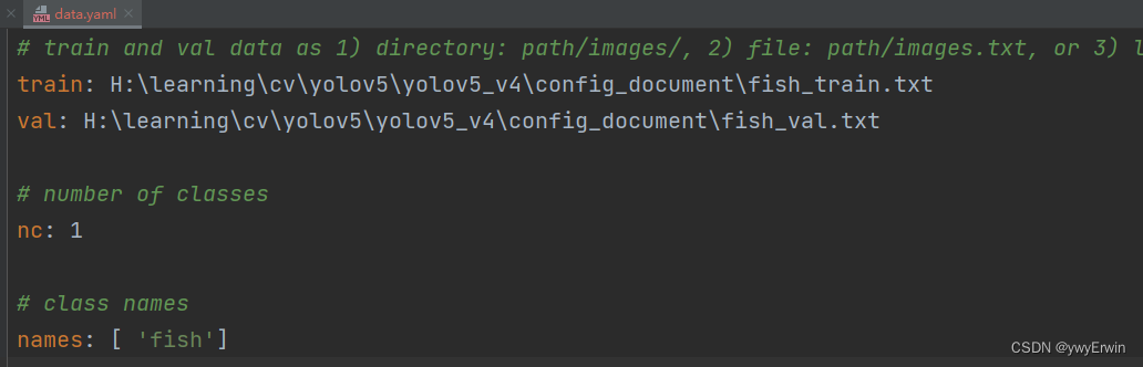
data.yaml 存放模型训练和验证路径,以及对应的类别数,类别名称:
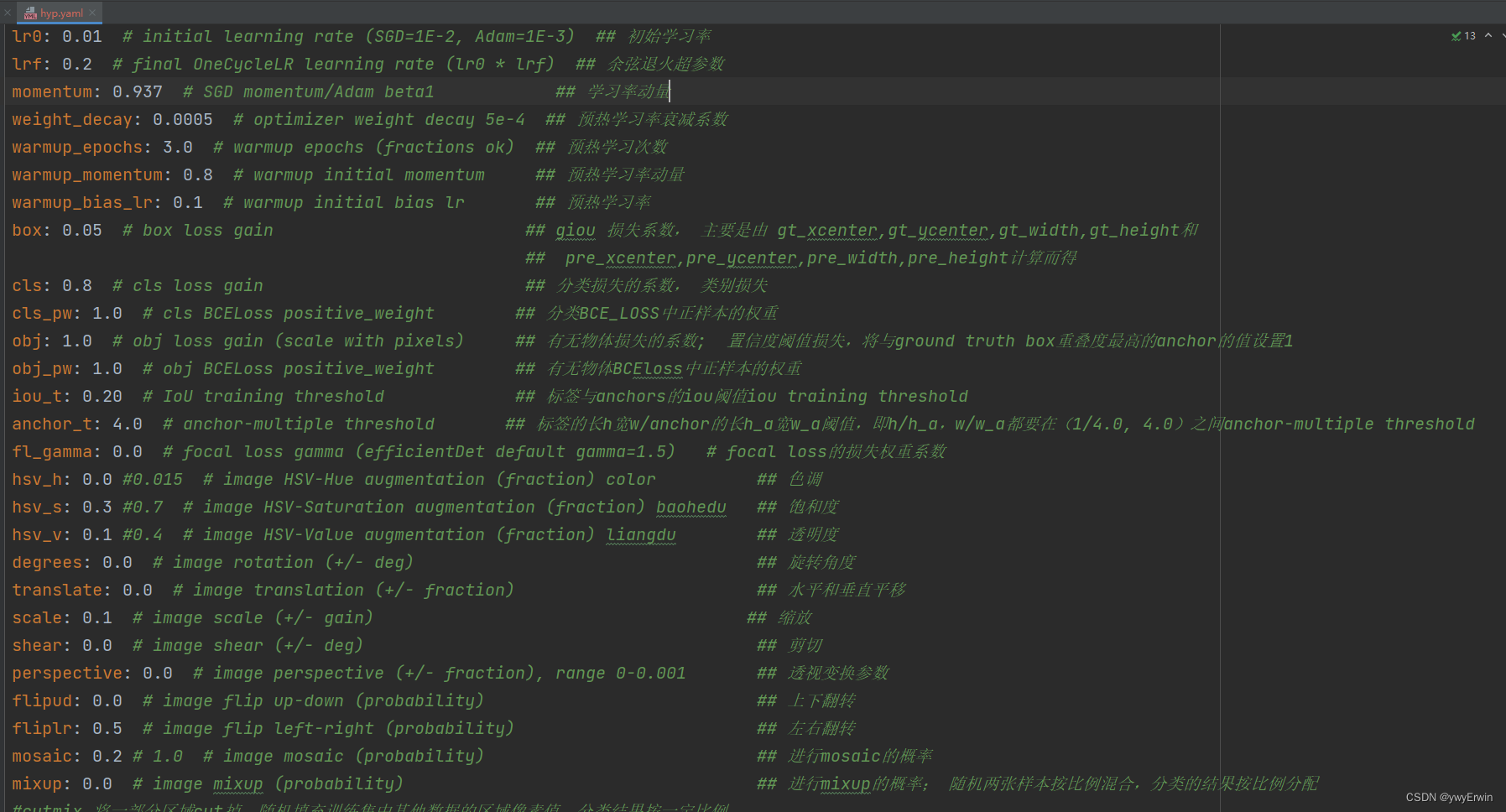
hyp.yaml为模型的配置参数,每个配置参数含义在其进行了简单的中文解释
yolov5l.yml和yolov5m.yml等分别为yolov5不同模型对应的架构,anchor,类别数和模型的宽度,深度。在训练模型过程中仅仅需要更改模型的类别数,对于Yolov5模型架构的设计,及不同大小模型的区别可以参考大白的一些博客,写的很详细,清晰。
二、训练代码详解
对于train.py文件的解读:
    # Directories
    wdir = save_dir / 'weights'
    wdir.mkdir(parents=True, exist_ok=True)  # make dir
    last = wdir / 'last.pt'
    best = wdir / 'best.pt'
    results_file = save_dir / 'results.txt'
设置最后需要保存的最好的(best)和最后的(last)的模型文件路径,以及验证集输出结果的txt文件路径,包含迭代的次数,占用显存大小,图片尺寸,精确率,召回率,位置损失,类别损失,置信度损失和map等。
    # Configure
    plots = not opt.evolve  # create plots
    cuda = device.type != 'cpu'
    init_seeds(2 + rank)
    with open(opt.data) as f:
        data_dict = yaml.load(f, Loader=yaml.FullLoader)  # data dict
    with torch_distributed_zero_first(rank):
        check_dataset(data_dict)  # check
    train_path = data_dict['train']
    test_path = data_dict['val']
    nc = 1 if opt.single_cls else int(data_dict['nc'])  # number of classes
    names = ['item'] if opt.single_cls and len(data_dict['names']) != 1 else data_dict['names']  # class names
    assert len(names) == nc, '%g names found for nc=%g dataset in %s' % (len(names), nc, opt.data)  # check assert True继续,False则终止程序运行

    # Model
通过读取data.yml配置文件,加载训练集和验证集数据路径(train_path, test_path),类别数和类别名称,可以将多类标签作为一类进行学习,即训练指令中加入–sing-cls
![]()
加载模型
    if pretrained:
        with torch_distributed_zero_first(rank):
            pass
            # attempt_download(weights)  # download if not found locally
        ckpt = torch.load(weights, map_location=device)  # load checkpoint
        # print('ckpt1', ckpt)
        if hyp.get('anchors'):
            ckpt['model'].yaml['anchors'] = round(hyp['anchors'])  # force autoanchor
        model = Model(opt.cfg or ckpt['model'].yaml, ch=3, nc=nc).to(device)  # create ch=3为输入通道数
        exclude = ['anchor'] if opt.cfg or hyp.get('anchors') else []  # exclude keys
        state_dict = ckpt['model'].float().state_dict()  # to FP32
        state_dict = intersect_dicts(state_dict, model.state_dict(), exclude=exclude)  # intersect
        model.load_state_dict(state_dict, strict=False)  # load
        logger.info('Transferred %g/%g items from %s' % (len(state_dict), len(model.state_dict()), weights))  # report
    else:
        model = Model(opt.cfg, ch=3, nc=nc).to(device)  # create
如果有预训练模型,则加载预训练模型,同时hyp.yaml中有anchors则获取其anchors
    # Freeze
    freeze = []  # parameter names to freeze (full or partial)
    for k, v in model.named_parameters():
        v.requires_grad = True  # train all layers
        if any(x in k for x in freeze):
            print('freezing %s' % k)
            v.requires_grad = False
设置需要冻结的层,即将模型的部分权重冻结,在模型训练过程中不会变化,只训练冻结层以为的权重参数。
    # Optimizer
    nbs = 64  # nominal batch size ;
    accumulate = max(round(nbs / total_batch_size), 1)  # accumulate loss before optimizing
    hyp['weight_decay'] *= total_batch_size * accumulate / nbs  # scale weight_decay
    logger.info(f"Scaled weight_decay = {hyp['weight_decay']}")

    pg0, pg1, pg2 = [], [], []  # optimizer parameter groups
    for k, v in model.named_modules():
        if hasattr(v, 'bias') and isinstance(v.bias, nn.Parameter):
            pg2.append(v.bias)  # biases
        if isinstance(v, nn.BatchNorm2d):
            pg0.append(v.weight)  # no decay
        elif hasattr(v, 'weight') and isinstance(v.weight, nn.Parameter):
            pg1.append(v.weight)  # apply decay
            # print('pg1', pg1)
这儿作者以batch-size为64为基准,若训练过程中batch-size大于64,则模型学习率衰减系数增大,如果训练过程batch-size小于64,则模型权重系数为hyp.yml中设置的值。因为batch-size大于64时,模型的批量数据的归一化更加稳定(批归一化:通过对图片三通道分别减批量数据的均值再除以方差),对于归一化稳定情况下可以增大学习率的速率,加速模型收敛。另外通过遍历模型的所有子层,将包含偏差,批归一化值和权重分别存放在pg0,pg1,pg2列表中
优化器
    if opt.adam:
        optimizer = optim.Adam(pg0, lr=hyp['lr0'], betas=(hyp['momentum'], 0.999))  # adjust beta1 to momentum
    else:
        optimizer = optim.SGD(pg0, lr=hyp['lr0'], momentum=hyp['momentum'], nesterov=True)

    optimizer.add_param_group({'params': pg1, 'weight_decay': hyp['weight_decay']})  # add pg1 with weight_decay
    optimizer.add_param_group({'params': pg2})  # add pg2 (biases)
    logger.info('Optimizer groups: %g .bias, %g conv.weight, %g other' % (len(pg2), len(pg1), len(pg0)))
    del pg0, pg1, pg2

    lf = one_cycle(1, hyp['lrf'], epochs)  # cosine 1->hyp['lrf']
    scheduler = lr_scheduler.LambdaLR(optimizer, lr_lambda=lf)
设置模型优化器,包括随机梯度下降(SGD)和自适应梯度下降(adam),将包含权重(pg1)和偏差(pg2)的层添加到优化器中,进而采用one_cycle和LambdaLR设置学习率衰减。模型训练过程中主要为权重和偏差的优化更新且学习率在warmup中先由小增大(一开始没有先验知识,需要小的学习率进行学习,以防学习过程陷入局部出不来。有一定先验知识进而将学习率增大,加速模型收敛,最后学习率再缓慢减少,因为最后模型已在最优区间,用小的学习率进行精进的优化)。
    start_epoch, best_fitness = 0, 0.0
    if pretrained:
        # Optimizer
        # print('ckpt2', ckpt)
        if ckpt['optimizer'] is not None:
            optimizer.load_state_dict(ckpt['optimizer'])
            best_fitness = ckpt['best_fitness']

        # Results
        if ckpt.get('training_results') is not None:
            with open(results_file, 'w') as file:
                file.write(ckpt['training_results'])  # write results.txt

        # Epochs
        start_epoch = ckpt['epoch'] + 1   # ckpt['epoch'] = -1
        if opt.resume:
            assert start_epoch > 0, '%s training to %g epochs is finished, nothing to resume.' % (weights, epochs)
        if epochs < start_epoch:
            logger.info('%s has been trained for %g epochs. Fine-tuning for %g additional epochs.' %
                        (weights, ckpt['epoch'], epochs))
            epochs += ckpt['epoch']  # finetune additional epochs

        del ckpt, state_dict
从预训练模型中加载保存的best_fitness,epoch,并将其作为训练模型的起始best_fitness和epoch(源码中默认为-1)
    gs = int(model.stride.max())  # grid size (max stride)
    nl = model.model[-1].nl  # number of detection layers (used for scaling hyp['obj']);
    imgsz, imgsz_test = [check_img_size(x, gs) for x in opt.img_size]  # verify imgsz are gs-multiples imgsz
gs为模型下采样最大的倍数,比如640×640分辨率下采样32倍为20(640/32=20)
nl为检测头输出的层数,为3层;
imgsz为图片分辨率大小
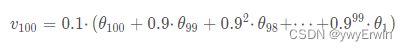
ema = ModelEMA(model) if rank in [-1, 0] else None ema为指数加权平均或滑动平均,其将前面模型训练权重,偏差进行保存,在本次训练过程中,假设为第n次,将第一次到第n-1次以指数权重进行加和,再加上本次的结果,且越远离第n次,指数系数越大,其所占的比重越小。采用指数加权平均的好处在于,模型不会因为某一次的权重好坏,将模型陷入局部状态,以n为100,指数系数为0.9为例,如下所示:
数据生成器
    dataloader, dataset = create_dataloader(train_path, imgsz, batch_size, gs, opt,
                                            hyp=hyp, augment=True, cache=opt.cache_images, rect=opt.rect, rank=rank,
                                            world_size=opt.world_size, workers=opt.workers,
                                            image_weights=opt.image_weights, quad=opt.quad)

    mlc = np.concatenate(dataset.labels, 0)[:, 0].max()  # max label class;
    nb = len(dataloader)  # number of batches
    assert mlc < nc, 'Label class %g exceeds nc=%g in %s. Possible class labels are 0-%g' % (mlc, nc, opt.data, nc - 1)
上述为数据生成器,通过数据生成器,将所有训练数据分成n个batch,对每一个batch的数据首先进行一系列数据增强(mosaic,mixup,随机裁剪,颜色变换,旋转等),对增强后的数据作为模型的输入。其中 rank:表示多张显卡训练时的进程编号;opt.world_size:表示总的进程数;opt.workers:表示加载数据时cpu的线程数;opt.image_weights:表示训练时,是否根据GT框的数量分布权重来选择图片,如果数据量多则权重大,被选到的次数多;opt.quad: dataloader 读取数据时, 是否使用collate_fn4来替代collate_fn。
在dataset.py程序中展现了数据生成器的原理和过程,其根据读取的训练数据路径,例如:txt格式,将所有数据路径保存在self.img_files。
    def cache_labels(self, path=Path('./labels.cache')):
        # Cache dataset labels, check images and read shapes
        x = {}  # dict
        nm, nf, ne, nc = 0, 0, 0, 0  # number missing, found, empty, duplicate
        pbar = tqdm(zip(self.img_files, self.label_files), desc='Scanning images', total=len(self.img_files))
        for i, (im_file, lb_file) in enumerate(pbar): ##  im_file是jpg,lb_file是txt带标签和坐标的
            try:
                # verify images
                im = Image.open(im_file)
                im.verify()  # PIL verify 验证图片是否损坏
                shape = exif_size(im)  # image size
                assert (shape[0] > 9) & (shape[1] > 9), 'image size <10 pixels'

                # verify labels
                if os.path.isfile(lb_file):
                    nf += 1  # label found 可以找到标签的
                    with open(lb_file, 'r') as f:
                        l = np.array([x.split() for x in f.read().strip().splitlines()], dtype=np.float32)  # labels
                    if len(l):
                        assert l.shape[1] == 5, 'labels require 5 columns each'
                        assert (l >= 0).all(), 'negative labels' #为负数的标签为错误的
                        assert (l[:, 1:] <= 1).all(), 'non-normalized or out of bounds coordinate labels'
                        assert np.unique(l, axis=0).shape[0] == l.shape[0], 'duplicate labels'
                    else:
                        ne += 1  # label empty 有txt,但txt文件里什么都没有,有xml文件的,但xml文件是空的

                        l = np.zeros((0, 5), dtype=np.float32)  ## 有xml文件,但没有标签的,加载标签为 [],空集
                else:
                    #没有txt的不加载
                    nm += 1  # label missing  没有txt,找不到标签的
                    l = np.zeros((0, 5), dtype=np.float32)

                x[im_file] = [l, shape] ##
except Exception as e:
                nc += 1
                print('WARNING: Ignoring corrupted image and/or label %s: %s' % (im_file, e))

            pbar.desc = f"Scanning '{path.parent / path.stem}' for images and labels... " \
                        f"{nf} found, {nm} missing, {ne} empty, {nc} corrupted"

        if nf == 0:
            print(f'WARNING: No labels found in {path}. See {help_url}')

        x['hash'] = get_hash(self.label_files + self.img_files)
        x['results'] = [nf, nm, ne, nc, i + 1]
        torch.save(x, path)  # save for next time
        logging.info(f"New cache created: {path}")
        return x
上述代码展示了将图片的标签和坐标读取,并查验是否包含有错误的标签文件(txt文件),例如每张图片对应的标签文件(txt)应该为5列,第一列为对应类别(0,1…),后四列为对应坐标,如果超过或不足5列就会报错;此外对于第一列(标签)只能为正数,如果为负则报错,对于后四列box的坐标是其相对整张图的比值,故其小于1,若大于1,则也会报错。对于没有txt或txt文件为空的,则其对应的标签和坐标设置为空集[],代码为: l = np.zeros((0, 5), dtype=np.float32),这样可以增加没有标签的数据作为负样本。
另外dataset.py中包含了所有的数据强例如mosaic,mixup,裁剪,旋转等,对应的配置参数为hyp.yml。
参数及类别权重
    # Model parameters
    hyp['cls'] *= nc / 80.  # scale hyp['cls'] to class count;
    hyp['obj'] *= imgsz ** 2 / 640. ** 2 * 3. / nl  # scale hyp['obj'] to image size and output layers
    model.nc = nc  # attach number of classes to model
    model.hyp = hyp  # attach hyperparameters to model
    model.gr = 1.0  # iou loss ratio (obj_loss = 1.0 or iou)
    model.class_weights = labels_to_class_weights(dataset.labels, nc).to(device) * nc  # attach class weights
    model.names = names
hyp['cls']和hyp['obj']分别为将类别损失系数基于coco数据集进行缩放和将图片缩放到对应输出层,因为配置文件中默认为训练coco数据集的配置参数。即自训练类别大于80,则类别损失加大,否则减少。labels_to_class_weights 定义如下:
def labels_to_class_weights(labels, nc=80):
    # Get class weights (inverse frequency) from training labels
    if labels[0] is None:  # no labels loaded
        return torch.Tensor()

    labels = np.concatenate(labels, 0)  # labels.shape = (866643, 5) for COCO
    classes = labels[:, 0].astype(np.int)  # labels = [class xywh]
    weights = np.bincount(classes, minlength=nc)  # occurrences per class; 每个类别的数量 ;例如:label [1,2,4,5,1] weights为 [0,2,1,0,1,1]

    weights[weights == 0] = 1  # replace empty bins with 1 ; 将类别数量为0的转为1
    weights = 1 / weights  # number of targets per class; 将每个类别的数量的倒数作为其权重值
    weights /= weights.sum()  # normalize ; 将每个类别的权重归一化
    return torch.from_numpy(weights)
其将每个类别的数量的倒数作为相应类别挑选图片的权重系数,例如:cat:20,dog:30,bird:10,则其类别权重系数分别为:20/60,30/60,10/60。
        # Update image weights (optional)
        if opt.image_weights:
            # Generate indices
            if rank in [-1, 0]:
                cw = model.class_weights.cpu().numpy() * (1 - maps) ** 2 / nc  # class weights; 每个类别的map,在测试的时候会更新,test.test时,对于map大的下次训练给予小的权重,map小的给予大的权重
                iw = labels_to_image_weights(dataset.labels, nc=nc, class_weights=cw)  # image weights;iw 每张图片被选中的权重,概率
                dataset.indices = random.choices(range(dataset.n), weights=iw, k=dataset.n)  # rand weighted idx;从所有的训练集中(依据索引),挑选所有训练集的图片,对应类别权重值大的循环多次挑选出,权重值小的,选出的次数少,甚至一次都不会选出
            # Broadcast if DDP
            if rank != -1:
                indices = (torch.tensor(dataset.indices) if rank == 0 else torch.zeros(dataset.n)).int()
                dist.broadcast(indices, 0)
                if rank != 0:
                    dataset.indices = indices.cpu().numpy()
若设置–img-weights,则对于每个batch的训练,其会更新相应的数据,通过每个类别的权重系数来随机选取相应类别的数据,如基于以上,cat:20,dog:30,bird:10,则其类别权重系数分别为:20/60,30/60,10/60。故而对类别cat的数据被当前batch选出的概率为1/3,通过每张图片的索引来选取。这样做的目的是保证了样本数较少的类别,其数据可以大概率的反复多次被挑选到,用于模型训练,加大模型对其特征的学习,拟合。
optimizer.zero_grad()优化器在进行下一次batch梯度的计算时,需要把上一次batch梯度信息设置为0,避免两次或多次相加。梯度值为最后的损失(loss)对权重(weights)的求导值。
warmup和前向传播
        for i, (imgs, targets, paths, _) in pbar:  # batch -------------------------------------------------------------
            ni = i + nb * epoch  # number integrated batches (since train start); ni为总的图片数量
            imgs = imgs.to(device, non_blocking=True).float() / 255.0  # uint8 to float32, 0-255 to 0.0-1.0

            # Warmup; nw: warmup总的图片数量
            if ni <= nw:
                xi = [0, nw]  # x interp
                # model.gr = np.interp(ni, xi, [0.0, 1.0])  # iou loss ratio (obj_loss = 1.0 or iou)
                accumulate = max(1, np.interp(ni, xi, [1, nbs / total_batch_size]).round())
                for j, x in enumerate(optimizer.param_groups):
                    # bias lr falls from 0.1 to lr0, all other lrs rise from 0.0 to lr0
                    x['lr'] = np.interp(ni, xi, [hyp['warmup_bias_lr'] if j == 2 else 0.0, x['initial_lr'] * lf(epoch)])
                    if 'momentum' in x:
                        x['momentum'] = np.interp(ni, xi, [hyp['warmup_momentum'], hyp['momentum']])

            # Forward
            with amp.autocast(enabled=cuda): ## 半精度计算,加快训练速度
                pred = model(imgs)  # forward
                loss, loss_items = compute_loss(pred, targets.to(device), model)  # loss scaled by batch_size
                # print('loss, loss_items', loss, loss_items)
                if rank != -1:
                    loss *= opt.world_size  # gradient averaged between devices in DDP mode
                if opt.quad:
                    loss *= 4.

            # Backward
            scaler.scale(loss).backward()
ni = i+nb*epoch为每一个epoch时batch数量的累加,nb为一个epoch总共的batch数量,比如:nb=10,对于第1个epoch,则epoch为0,ni=i,ni为训练时的batch数量,对于第二个epoch,epoch=1,前面已经有了nb*epoch=1*10=10个batch,现在每次再原来10个batch的基础上累加。
if ni<nw,为当前的batch小于设置的warmup的总的batch数(warmup的epoch*nb),则进行warmup,学习率先小再缓慢增加,进行先验知识的学习。
#forward 前向传播,进行损失函数(基于预测值pred,目标值targets)的计算,imgs.to(device)和 targets.to(device)为将图片数据和目标值放入设备(GPU或CPU)计算。其损失函数的计算如下所示:
损失函数计算
def compute_loss(p, targets, model):  # predictions, targets, model
    device = targets.device
    lcls, lbox, lobj = torch.zeros(1, device=device), torch.zeros(1, device=device), torch.zeros(1, device=device)
    tcls, tbox, indices, anchors = build_targets(p, targets, model)  # targets tcls (3,808)表示3个检测头对应的gt box的类别, tobox (3,([808,4]))表示3个检测头对应的gt box的xywh; 808 表示808个框
    # anchors (3,([802,2])),表示每个检测头对应的808个gt box所对应的anchor
    h = model.hyp  # hyperparameters

    # Define criteria
    BCEcls = nn.BCEWithLogitsLoss(pos_weight=torch.tensor([h['cls_pw']], device=device))  # weight=model.class_weights)  其将nn.sigmoid()和nn.BCELoss()合并在一起了
    BCEobj = nn.BCEWithLogitsLoss(pos_weight=torch.tensor([h['obj_pw']], device=device))

    # Class label smoothing https://arxiv.org/pdf/1902.04103.pdf eqn 3
    cp, cn = smooth_BCE(eps=0.0)

    # Focal loss
    g = h['fl_gamma']  # focal loss gamma
    if g > 0:
        BCEcls, BCEobj = FocalLoss(BCEcls, g), FocalLoss(BCEobj, g)
    # Losses
    nt = 0  # number of targets
    no = len(p)  # number of outputs ; 最后输出的三层 no=3
    balance = [4.0, 1.0, 0.3, 0.1, 0.03]  # P3-P7  置信度损失这儿为什么[80 80]需要乘以 4.0
    for i, pi in enumerate(p):  # layer index, layer predictions, 预测的三层,i仅为0,1,2 预测头[80 80]  [40 40]  [20 20]
        b, a, gj, gi = indices[i]  # image, anchor, gridy, gridx
        tobj = torch.zeros_like(pi[..., 0], device=device)  # target obj
        n = b.shape[0]  # number of targets   targets[]
        if n:
            nt += n  # cumulative targets
            ps = pi[b, a, gj, gi]  # prediction subset corresponding to targets
            # Regression
            pxy = ps[:, :2].sigmoid() * 2. - 0.5
            pwh = (ps[:, 2:4].sigmoid() * 2) ** 2 * anchors[i]
            pbox = torch.cat((pxy, pwh), 1)  # predicted box
            iou = bbox_iou(pbox.T, tbox[i], x1y1x2y2=False, CIoU=True)  # iou(prediction, target)  ##  可以对比一下GIOU, CIOU, DIOU的区别与各自的作用
            lbox += (1.0 - iou).mean()  # iou loss,因为是损失,所以需要为负,或者越小越好
            # Objectness
            tobj[b, a, gj, gi] = (1.0 - model.gr) + model.gr * iou.detach().clamp(0).type(tobj.dtype)  # iou ratio  置信度预测

            if model.nc > 1:  # cls loss (only if multiple classes); ps[:, 5:] 对应三个类别, 多个类别才需要执行
                t = torch.full_like(ps[:, 5:], cn, device=device)  # targets

                t[range(n), tcls[i]] = cp

                lcls += BCEcls(ps[:, 5:], t)  # BCE

        lobj += BCEobj(pi[..., 4], tobj) * balance[i]  # obj loss
        # print("lobj", lobj)
    s = 3 / no  # output count scaling
    lbox *= h['box'] * s
    lobj *= h['obj']
    lcls *= h['cls'] * s
    bs = tobj.shape[0]  # batch size tobj [batch-size 3 80 80 ] [batch-size 3 40 40 ]  [batch-size 3 20 20 ]
    loss = lbox + lobj + lcls
    ## 最后需要乘以bs,即批次数量
    return loss * bs, torch.cat((lbox, lobj, lcls, loss)).detach()
其对类别损失和置信度损失采用先进行sigmoid计算,再采用交叉熵计算;如果要增加focal loss需要在hyp.yml中将fl_gamma设置为一个大于0的值(focal loss权重系数),focalloss公式如下![]() ,其设计的目的一方面通过α平衡正负样本,文中默认α为0.25,则正样本权重为0.25,负样本权重为0.75,增加了负样本的权重。另一方面,通过γ来调节难易样本的损失权重,比如γ=2,当dog1的概率p为0.9时,其损失权重为(1-0.9)^2为0.01,当其概率为0.1时,其损失权重为(1-0.1)^2为0.81。故加大了对检测概率较低,难以识别的类别的损失权重。对于
,其设计的目的一方面通过α平衡正负样本,文中默认α为0.25,则正样本权重为0.25,负样本权重为0.75,增加了负样本的权重。另一方面,通过γ来调节难易样本的损失权重,比如γ=2,当dog1的概率p为0.9时,其损失权重为(1-0.9)^2为0.01,当其概率为0.1时,其损失权重为(1-0.1)^2为0.81。故加大了对检测概率较低,难以识别的类别的损失权重。对于
cp, cn = smooth_BCE(eps=0.0) 为对每个类别进行label smooth,目的是保留不同类别相似特征的信息。不至于绝对化,采用这种方式一般可以提升整体准确性,但loss会相对较大。(比如:dog1:0.98 cat1:0.02,采用labelsmooth后dog1:0.88,cat1:0.12)最后box的位置损失采用IOU的形式,也可以做IOU的变体GIOU或CIOU。
准确性和召回率计算
        # DDP process 0 or single-GPU
        if rank in [-1, 0]:
            # mAP
            if ema:
                ema.update_attr(model, include=['yaml', 'nc', 'hyp', 'gr', 'names', 'stride', 'class_weights'])
            final_epoch = epoch + 1 == epochs
            if not opt.notest or final_epoch:  # Calculate mAP
                results, maps, times = test.test(opt.data,
                                                 batch_size=total_batch_size,
                                                 imgsz=imgsz_test,
                                                 model=ema.ema,
                                                 single_cls=opt.single_cls,
                                                 dataloader=testloader,
                                                 save_dir=save_dir,
                                                 plots=plots and final_epoch,
                                                 log_imgs=opt.log_imgs if wandb else 0)
rank为[-1,0]为进行单机模式,通过test.test来计算验证集数据的准确性,召回率,map,过程如下:
①首先将模型框架参数固定,进行推理模式(model.eval()和with torch.no_grad()),对输入的图片做前处理(一般标准归一化或归一化);
②对模型预测的结果基于IOU进行非极大值抑制(nms)
③对nms后剩余的box(标签,坐标)和正样本的box进行比较,文章中选择IOU从0.5–0.95(间隔0.05),十个点进行准确性和召回率的统计,当预测box和实际box的IOU大于设定阈值且预测类别一致为正确的,反之为错误的。最后准确性和召回率为这十个设定IOU的统计结果的平均值。
if len(stats) and stats[0].any():
    p, r, ap, f1, ap_class = ap_per_class(*stats, plot=plots, save_dir=save_dir, names=names)
    p, r, ap50, ap = p[:, 0], r[:, 0], ap[:, 0], ap.mean(1)  # [P, R, AP@0.5, AP@0.5:0.95]
    ## 计算了IOU从0.5到0.95时准确性和召回率分别为多少,并进行了平均值的计算
    mp, mr, map50, map = p.mean(), r.mean(), ap50.mean(), ap.mean()
    nt = np.bincount(stats[3].astype(np.int64), minlength=nc)  # number of targets per class
else:
    nt = torch.zeros(1)
            # Update best mAP
            fi = fitness(np.array(results).reshape(1, -1))  # weighted combination of [P, R, mAP@.5, mAP@.5-.95]

            if fi > best_fitness:
                best_fitness = fi
            # Save model
            save = (not opt.nosave) or (final_epoch and not opt.evolve)
            if save:
                with open(results_file, 'r') as f:  # create checkpoint
                    ckpt = {'epoch': epoch,
                            'best_fitness': best_fitness,
                            'training_results': f.read(),
                            'model': ema.ema,
                            'optimizer': None if final_epoch else optimizer.state_dict(),
                            'wandb_id': wandb_run.id if wandb else None}

                # Save last, best and delete
                torch.save(ckpt, last)
                if best_fitness == fi:
                    torch.save(ckpt, best)
                del ckpt
最后对于验证集的结果与上次进行比较,保存每次map较大的作为best,并保存其模型文件,同时保存最后训练模型的pt文件。
第一次写博客,写的不好的地方欢迎留言指正!
文章出处登录后可见!