前言
2021年8月19日 订正部分原理
在上次的文章中我们解析了backbone网络的构建源码,在这篇中我们针对yolo.py剩余的部分进行debug解析。如果没看过之前文章的小伙伴,推荐先查看这个系列的第一篇和第二篇。下面贴上传送门:
1.yolov5源码解析第一篇 架构设计和debug准备
2.yolov5源码解析第二篇 backbone源码解析
今天我们继续对model.py里的Detect类进行解析,这部分对应yolov5的检查头部分。
detect类在model.py里,这部分代码如下:
class Detect(nn.Module):
    stride = None  # strides computed during build
    export = False  # onnx export

    def __init__(self, nc=80, anchors=(), ch=()):  # detection layer
        super(Detect, self).__init__()
        self.nc = nc  # number of classes
        self.no = nc + 5  # number of outputs per anchor  85 for coco
        self.nl = len(anchors)  # number of detection layers 3
        self.na = len(anchors[0]) // 2  # number of anchors  3
        self.grid = [torch.zeros(1)] * self.nl  # init grid
        a = torch.tensor(anchors).float().view(self.nl, -1, 2)
        self.register_buffer('anchors', a)  # shape(nl,na,2)
        self.register_buffer('anchor_grid', a.clone().view(self.nl, 1, -1, 1, 1, 2))  # shape(nl,1,na,1,1,2)
        self.m = nn.ModuleList(nn.Conv2d(x, self.no * self.na, 1) for x in ch)  # output conv 128=>255/256=>255/512=>255

    def forward(self, x):
        # x = x.copy()  # for profiling
        z = []  # inference output
        self.training |= self.export
        for i in range(self.nl):
            x[i] = self.m[i](x[i])  # conv
            bs, _, ny, nx = x[i].shape  # x(bs,255,20,20) to x(bs,3,20,20,85)
            x[i] = x[i].view(bs, self.na, self.no, ny, nx).permute(0, 1, 3, 4, 2).contiguous()

            if not self.training:  # inference
                if self.grid[i].shape[2:4] != x[i].shape[2:4]:
                    self.grid[i] = self._make_grid(nx, ny).to(x[i].device)

                y = x[i].sigmoid()
                y[..., 0:2] = (y[..., 0:2] * 2. - 0.5 + self.grid[i].to(x[i].device)) * self.stride[i]  # xy
                y[..., 2:4] = (y[..., 2:4] * 2) ** 2 * self.anchor_grid[i]  # wh
                z.append(y.view(bs, -1, self.no))

        return x if self.training else (torch.cat(z, 1), x)

    @staticmethod
    def _make_grid(nx=20, ny=20):
        yv, xv = torch.meshgrid([torch.arange(ny), torch.arange(nx)])
        return torch.stack((xv, yv), 2).view((1, 1, ny, nx, 2)).float()
我们首先来看这个类的__init__()函数:
    def __init__(self, nc=80, anchors=(), ch=()):  # detection layer
        super(Detect, self).__init__()
        self.nc = nc  # number of classes
        self.no = nc + 5  # number of outputs per anchor  85 for coco
        self.nl = len(anchors)  # number of detection layers 3
        self.na = len(anchors[0]) // 2  # number of anchors  3
        self.grid = [torch.zeros(1)] * self.nl  # init grid
        a = torch.tensor(anchors).float().view(self.nl, -1, 2)
        self.register_buffer('anchors', a)  # shape(nl,na,2)
        self.register_buffer('anchor_grid', a.clone().view(self.nl, 1, -1, 1, 1, 2))  # shape(nl,1,na,1,1,2)
        self.m = nn.ModuleList(nn.Conv2d(x, self.no * self.na, 1) for x in ch)  # output conv 128=>255/256=>255/512=>255
yolov5的检测头仍为FPN结构,所以self.m为3个输出卷积。这三个输出卷积模块的channel变化分别为128=>255|256=>255|512=>255。
self.no为每个anchor位置的输出channel维度,每个位置都预测80个类(coco)+ 4个位置坐标xywh + 1个confidence score。所以输出channel为85。每个尺度下有3个anchor位置,所以输出85*3=255个channel。
下面我们再来看下head部分的forward()函数:
    def forward(self, x):
        # x = x.copy()  # for profiling
        z = []  # inference output
        self.training |= self.export
        for i in range(self.nl):
            x[i] = self.m[i](x[i])  # conv
            bs, _, ny, nx = x[i].shape  # x(bs,255,20,20) to x(bs,3,20,20,85)
            x[i] = x[i].view(bs, self.na, self.no, ny, nx).permute(0, 1, 3, 4, 2).contiguous()

            if not self.training:  # inference
                if self.grid[i].shape[2:4] != x[i].shape[2:4]:
                    self.grid[i] = self._make_grid(nx, ny).to(x[i].device)

                y = x[i].sigmoid()
                y[..., 0:2] = (y[..., 0:2] * 2. - 0.5 + self.grid[i].to(x[i].device)) * self.stride[i]  # xy
                y[..., 2:4] = (y[..., 2:4] * 2) ** 2 * self.anchor_grid[i]  # wh
                z.append(y.view(bs, -1, self.no))

        return x if self.training else (torch.cat(z, 1), x)
x是一个列表的形式,分别对应着3个head的输入。它们的shape分别为:
- [B, 128, 32, 32]
- [B, 256, 16, 16]
- [B, 512, 8, 8]
三个输入先后被送入了3个卷积,得到输出结果。
x[i] = x[i].view(bs, self.na, self.no, ny, nx).permute(0, 1, 3, 4, 2).contiguous()
这里将x进行变换从:
- x[0]:(bs,255,32,32) => x(bs,3,32,32,85)
- x[1]:(bs,255,32,32) => x(bs,3,16,16,85)
- x[2]:(bs,255,32,32) => x(bs,3,8,8,85)
            if not self.training:  # inference
                if self.grid[i].shape[2:4] != x[i].shape[2:4]:
                    self.grid[i] = self._make_grid(nx, ny).to(x[i].device)
    def _make_grid(nx=20, ny=20):
        yv, xv = torch.meshgrid([torch.arange(ny), torch.arange(nx)])
        return torch.stack((xv, yv), 2).view((1, 1, ny, nx, 2)).float()
这里的_make_grid()函数是准备好格点。所有的预测的单位长度都是基于grid层面的而不是原图。注意每一层的grid的尺寸都是不一样的,和每一层输出的尺寸w,h是一样的。
   y = x[i].sigmoid()
   y[..., 0:2] = (y[..., 0:2] * 2. - 0.5 + self.grid[i].to(x[i].device)) * self.stride[i]  # xy
   y[..., 2:4] = (y[..., 2:4] * 2) ** 2 * self.anchor_grid[i]  # wh
   z.append(y.view(bs, -1, self.no))
这里是inference的核心代码,我们要好好剖析一下,相比于yolov3,yolov5有一些变化:
yolov3的bbox回归机制如下图所示: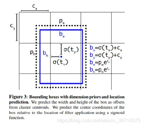
而yolov5的回归机制如下图所示: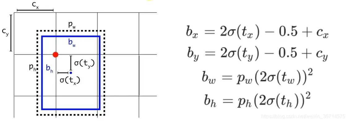
y[..., 0:2] = (y[..., 0:2] * 2. - 0.5 + self.grid[i].to(x[i].device)) * self.stride[i]
这里可以明显发现box center的x,y的预测被乘以2并减去了0.5,所以这里的值域从yolov3里的(0,1)注意是开区间,变成了(-0.5, 1.5)。
从表面理解是yolov5可以跨半个格点预测了,这样可以提高对格点周围的bbox的召回。当然还有一个好处就是也解决了yolov3中因为sigmoid开区间而导致中心无法到达边界处的问题。这里是我分析的观点,如果读者有其他的思路欢迎留言点拨。
同理,在w,h的回归上,yolov5也有了新的变化:
y[..., 2:4] = (y[..., 2:4] * 2) ** 2 * self.anchor_grid[i]
这里是预测boundingbox的wh。先回顾下yolov3里的预测:
        x = torch.sigmoid(prediction[..., 0])  # Center x  #B A H W
        y = torch.sigmoid(prediction[..., 1])  # Center y  #B A H W
        w = prediction[..., 2]  # Width                    #B A H W
        h = prediction[..., 3]  # Height                   #B A H W
        pred_conf = torch.sigmoid(prediction[..., 4])  # Conf
        pred_cls = torch.sigmoid(prediction[..., 5:])  # Cls pred.
很明显yolov3对于w,h没有做sigmoid,而在yolov5中对于x,y,w,h都做了sigmoid。其次yolov5的预测缩放比例变成了:(2*w_pred/h_pred) ^2。
值域从基于anchor宽高的(0,+∞)变成了(0,4)。这里我的理解是这个预测的框范围更精准了,通过sigmoid约束,让回归的框比例尺寸更为合理。和上面一样,这里是我分析的观点,如果读者有其他的思路欢迎留言点拨。
到这里我们就分析完了Detect类里面的所有代码。下面我回到Model类里面,最后分析它的前向传播过程,这里有两个函数forward()和forward_once()两个函数:
    def forward_once(self, x, profile=False):
        y, dt = [], []  # outputs
        for m in self.model:
            if m.f != -1:  # if not from previous layer
                x = y[m.f] if isinstance(m.f, int) else [x if j == -1 else y[j] for j in m.f]  # from earlier layers

            if profile:
                o = thop.profile(m, inputs=(x,), verbose=False)[0] / 1E9 * 2 if thop else 0  # FLOPS
                t = time_synchronized()
                for _ in range(10):
                    _ = m(x)
                dt.append((time_synchronized() - t) * 100)
                print('%10.1f%10.0f%10.1fms %-40s' % (o, m.np, dt[-1], m.type))

            x = m(x)  # run
            y.append(x if m.i in self.save else None)  # save output

        if profile:
            print('%.1fms total' % sum(dt))
        return x
self.foward_once()就是前向执行一次model里的所有module,得到结果。profile参数打开会记录每个模块的平均执行时长和flops用于分析模型的瓶颈,提高模型的执行速度和降低显存占用。
    def forward(self, x, augment=False, profile=False):
        if augment:
            img_size = x.shape[-2:]  # height, width
            s = [1, 0.83, 0.67]  # scales
            f = [None, 3, None]  # flips (2-ud, 3-lr)
            y = []  # outputs
            for si, fi in zip(s, f):
                xi = scale_img(x.flip(fi) if fi else x, si, gs=int(self.stride.max()))
                yi = self.forward_once(xi)[0]  # forward
                # cv2.imwrite(f'img_{si}.jpg', 255 * xi[0].cpu().numpy().transpose((1, 2, 0))[:, :, ::-1])  # save
                yi[..., :4] /= si  # de-scale
                if fi == 2:
                    yi[..., 1] = img_size[0] - 1 - yi[..., 1]  # de-flip ud
                elif fi == 3:
                    yi[..., 0] = img_size[1] - 1 - yi[..., 0]  # de-flip lr
                y.append(yi)
            return torch.cat(y, 1), None  # augmented inference, train
        else:
            return self.forward_once(x, profile)  # single-scale inference, train
self.forward()函数里面augment可以理解为控制TTA,如果打开会对图片进行scale和flip。默认是关闭的。
def scale_img(img, ratio=1.0, same_shape=False, gs=32):  # img(16,3,256,416)
    # scales img(bs,3,y,x) by ratio constrained to gs-multiple
    if ratio == 1.0:
        return img
    else:
        h, w = img.shape[2:]
        s = (int(h * ratio), int(w * ratio))  # new size
        img = F.interpolate(img, size=s, mode='bilinear', align_corners=False)  # resize
        if not same_shape:  # pad/crop img
            h, w = [math.ceil(x * ratio / gs) * gs for x in (h, w)]
        return F.pad(img, [0, w - s[1], 0, h - s[0]], value=0.447)  # value = imagenet mean
scale_img的源码如上,就是通过普通的双线性插值实现,根据ratio来控制图片的缩放比例,最后通过pad 0补齐到原图的尺寸。
至此整个yolov5 head的前向传播和inference的源码就分析完了。整个实现debug下来感觉也是比较通俗易懂的,整体上yolov3的差距也不是特别大。
在下一篇我们会开始分析重点分析yolov5的train.py,既剖析yolov5的训练过程。谢谢大家阅读!
版权声明:本文为博主吸欧大王原创文章,版权归属原作者,如果侵权,请联系我们删除!
原文链接:https://blog.csdn.net/weixin_36714575/article/details/114238645