【玩转yolov5】之anchor匹配策略(build_targets)分析(1)

这里我们实际推演一下yolov5训练过程中的anchor匹配策略,为了简化数据和便于理解，设定以下训练参数。

• 输入分辨率(img-size)：608×608
• 分类数(num_classes)：2
• batchsize：1
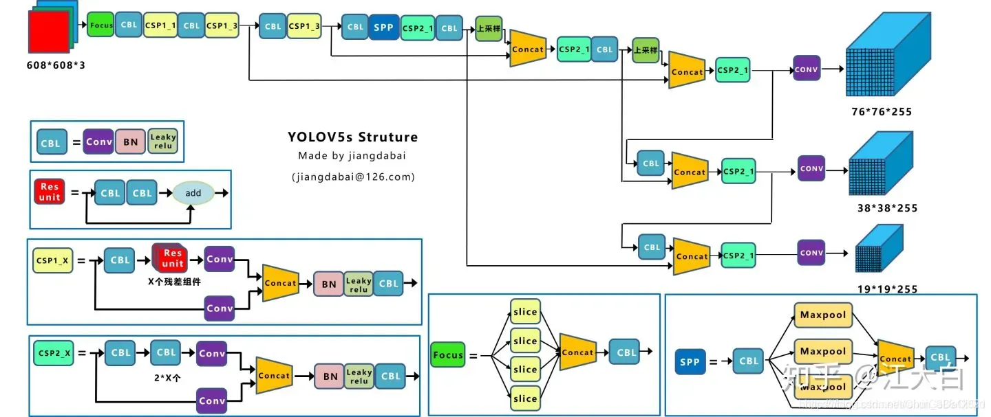
• 网络结构如下图所示：

def build_targets(pred, targets, model):
    """
    pred:
    type(pred) : <class 'list'>
    """
    #p:predict,targets:gt
    # Build targets for compute_loss(), input targets(image,class,x,y,w,h)
    det = model.module.model[-1] if is_parallel(model) else model.model[-1]  # Detect() module

输入参数pred为网络的预测输出，它是一个list包含三个检测头的输出tensor。

(Pdb) print(type(pred))

(Pdb) print(len(pred))
3
(Pdb) print(pred[0].shape)
torch.Size([1, 3, 76, 76, 7])  #1：batch-size,3:该层anchor的数量,7:位置(4),obj(1),分类(2)
(Pdb) print(pred[1].shape)
torch.Size([1, 3, 38, 38, 7])
(Pdb) print(pred[2].shape)
torch.Size([1, 3, 19, 19, 7])

targets为标签信息(gt)，我这里只有一张图片,包含14个gt框,且类别id为0,在我自己的训练集里面类别0表示行人。其中第1列为图片在当前batch的id号，第2列为类别id，后面依次是归一化了的gt框的x,y,w,h坐标。

(Pdb) print(targets.shape)
torch.Size([14, 6])
(Pdb) print(targets)
tensor([[0.00000, 0.00000, 0.56899, 0.42326, 0.46638, 0.60944],
[0.00000, 0.00000, 0.27361, 0.59615, 0.02720, 0.02479],
[0.00000, 0.00000, 0.10139, 0.59295, 0.04401, 0.03425],
[0.00000, 0.00000, 0.03831, 0.59863, 0.06223, 0.02805],
[0.00000, 0.00000, 0.04395, 0.57031, 0.02176, 0.06153],
[0.00000, 0.00000, 0.13498, 0.57074, 0.01102, 0.03152],
[0.00000, 0.00000, 0.25948, 0.59213, 0.01772, 0.03131],
[0.00000, 0.00000, 0.29733, 0.63080, 0.07516, 0.02536],
[0.00000, 0.00000, 0.16594, 0.57749, 0.33188, 0.13282],
[0.00000, 0.00000, 0.79662, 0.89971, 0.40677, 0.20058],
[0.00000, 0.00000, 0.14473, 0.96773, 0.01969, 0.03341],
[0.00000, 0.00000, 0.10170, 0.96792, 0.01562, 0.03481],
[0.00000, 0.00000, 0.27727, 0.95932, 0.03071, 0.07851],
[0.00000, 0.00000, 0.18102, 0.98325, 0.00749, 0.01072]])

model自然就是表示的模型，det是模型的检测头，从该对象中可以拿到anchor数量(na)以及尺寸,检测头数量(nl)等信息。

    na, nt = det.na, targets.shape[0]  # number of anchors, targets
    tcls, tbox, indices, anch = [], [], [], []
    gain = torch.ones(7, device=targets.device)  # normalized to gridspace gain
    ai = torch.arange(na, device=targets.device).float().view(na, 1).repeat(1, nt)  # same as .repeat_interleave(nt)
    targets = torch.cat((targets.repeat(na, 1, 1), ai[:, :, None]), 2) 

这里的骚操作还挺多，pytorch不熟练的话only look once还真看不明白，我稍微拆解一下。

(Pdb) na,nt,gain
(3, 14, tensor([1., 1., 1., 1., 1., 1., 1.]))
(Pdb) torch.arange(na).float().view(na,1)
tensor([[0.],
[1.],
[2.]])
(Pdb) torch.arange(na).float().view(na,1).repeat(1,nt) #第二个维度复制nt遍
tensor([[0., 0., 0., 0., 0., 0., 0., 0., 0., 0., 0., 0., 0., 0.],
[1., 1., 1., 1., 1., 1., 1., 1., 1., 1., 1., 1., 1., 1.],
[2., 2., 2., 2., 2., 2., 2., 2., 2., 2., 2., 2., 2., 2.]])

(Pdb) targets.shape
torch.Size([14, 6])
(Pdb) targets.repeat(na,1,1).shape #targets原本只有两维,该repeat操作过后会增加一维。
torch.Size([3, 14, 6])

(Pdb) ai[:,:,None].shape #原本两维的ai也会增加一维
torch.Size([3, 14, 1])

(Pdb)  torch.cat((targets.repeat(na, 1, 1), ai[:, :, None]), 2).shape #两个3维的tensort在第2维上concat
torch.Size([3, 14, 7])

(Pdb)  torch.cat((targets.repeat(na, 1, 1), ai[:, :, None]), 2)
tensor([[[0.00000, 0.00000, 0.56899, 0.42326, 0.46638, 0.60944, 0.00000],
[0.00000, 0.00000, 0.27361, 0.59615, 0.02720, 0.02479, 0.00000],
[0.00000, 0.00000, 0.10139, 0.59295, 0.04401, 0.03425, 0.00000],
…]，

[[0.00000, 0.00000, 0.56899, 0.42326, 0.46638, 0.60944, 1.00000],
[0.00000, 0.00000, 0.27361, 0.59615, 0.02720, 0.02479, 1.00000],
…]，

[[0.00000, 0.00000, 0.56899, 0.42326, 0.46638, 0.60944, 2.00000],
[0.00000, 0.00000, 0.27361, 0.59615, 0.02720, 0.02479, 2.00000],
…]])

    g = 0.5  # bias
    off = torch.tensor([[0, 0],
                        [1, 0], [0, 1], [-1, 0], [0, -1],  # j,k,l,m
                        # [1, 1], [1, -1], [-1, 1], [-1, -1],  # jk,jm,lk,lm
                        ], device=targets.device).float() * g  # offsets

off是偏置矩阵。

(Pdb) print(off)
tensor([[ 0.00000,  0.00000],
[ 0.50000,  0.00000],
[ 0.00000,  0.50000],
[-0.50000,  0.00000],
[ 0.00000, -0.50000]])

 for i in range(det.nl): #nl=>3
        anchors = det.anchors[i] #shape=>[3,3,2]
        gain[2:6] = torch.tensor(pred[i].shape)[[3, 2, 3, 2]]  
        # Match targets to anchors
        t = targets * gain

det.nl为预测层也就是检测头的数量，anchor匹配需要逐层进行。不同的预测层其特征图的尺寸不一样,而targets是相对于输入分辨率的宽和高作了归一化，targets*gain通过将归一化的box乘以特征图尺度从而将box坐标投影到特征图上。

(Pdb) pred[0].shape
torch.Size([1, 3, 76, 76, 7])  #1,3,h,w,7
(Pdb) torch.tensor(pred[0].shape)[[3,2,3,2]]
tensor([76, 76, 76, 76])

          if nt:
                # Matches
                r = t[:, :, 4:6] / anchors[:, None]  # wh ratio
                j = torch.max(r, 1. / r).max(2)[0] < model.hyp['anchor_t']  # compare
                # j = wh_iou(anchors, t[:, 4:6]) > model.hyp['iou_t']  # iou(3,n)=wh_iou(anchors(3,2), gwh(n,2))
                t = t[j]  # filter

yolov5抛弃了MaxIOU匹配规则而采用shape匹配规则，计算标签box和当前层的anchors的宽高比，即:wb/wa,hb/ha。如果宽高比大于设定的阈值说明该box没有合适的anchor，在该预测层之间将这些box当背景过滤掉(是个狠人!)。

(Pdb) torch.max(r,1./r).shape
torch.Size([3, 14, 2])
(Pdb) torch.max(r,1./r).max(2) #返回两组值,values和indices
torch.return_types.max(
values=tensor([[28.50301,  1.65375,  2.67556,  3.78370,  2.87777,  1.49309,  1.46451,  4.56943, 20.17829, 24.73137,  1.56263,  1.62791,  3.67186,  2.19651],
[17.72234,  1.99010,  1.67222,  2.36481,  1.24703,  2.38895,  1.57575,  2.85589, 12.61143, 15.45711,  1.47680,  1.68486,  1.59114,  4.60130],
[16.11040,  1.99547,  1.23339,  1.34871,  2.49381,  4.92720,  3.06377,  1.49178,  6.11463,  7.49436,  2.75656,  3.47502,  2.07540,  7.24849]]),
indices=tensor([[1, 0, 0, 0, 1, 0, 1, 0, 0, 0, 1, 1, 1, 0],
[0, 1, 0, 0, 1, 0, 1, 0, 0, 0, 1, 0, 1, 1],
[1, 0, 0, 1, 0, 0, 0, 1, 0, 0, 0, 0, 1, 0]]))
(Pdb) torch.max(r,1./r).max(2)[0] < model.hyp[‘anchor_t’]
tensor([[False,  True,  True,  True,  True,  True,  True, False, False, False,  True,  True,  True,  True],
[False,  True,  True,  True,  True,  True,  True,  True, False, False,  True,  True,  True, False],
[False,  True,  True,  True,  True, False,  True,  True, False, False,  True,  True,  True, False]])
(Pdb) print(j.shape)
torch.Size([3, 14])
(Pdb) print(t.shape)
torch.Size([3, 14, 7])
(Pdb) t[j].shape
torch.Size([29, 7])
(Pdb) t[j]
tensor([[ 0.00000,  0.00000, 20.79421, 45.30740,  2.06718,  1.88433,  0.00000],
[ 0.00000,  0.00000,  7.70598, 45.06429,  3.34444,  2.60274,  0.00000],
[ 0.00000,  0.00000,  2.91188, 45.49583,  4.72962,  2.13167,  0.00000],
[ 0.00000,  0.00000,  3.34012, 43.34355,  1.65410,  4.67637,  0.00000],
[ 0.00000,  0.00000, 10.25882, 43.37595,  0.83719,  2.39581,  0.00000],
[ 0.00000,  0.00000, 19.72059, 45.00159,  1.34638,  2.37982,  0.00000],
[ 0.00000,  0.00000, 10.99985, 73.54744,  1.49643,  2.53927,  0.00000],
[ 0.00000,  0.00000,  7.72917, 73.56174,  1.18704,  2.64536,  0.00000],
[ 0.00000,  0.00000, 21.07247, 72.90799,  2.33363,  5.96677,  0.00000],
[ 0.00000,  0.00000, 13.75753, 74.72697,  0.56908,  0.81499,  0.00000],
[ 0.00000,  0.00000, 20.79421, 45.30740,  2.06718,  1.88433,  1.00000],
[ 0.00000,  0.00000,  7.70598, 45.06429,  3.34444,  2.60274,  1.00000],
[ 0.00000,  0.00000,  2.91188, 45.49583,  4.72962,  2.13167,  1.00000],
[ 0.00000,  0.00000,  3.34012, 43.34355,  1.65410,  4.67637,  1.00000],
[ 0.00000,  0.00000, 10.25882, 43.37595,  0.83719,  2.39581,  1.00000],
[ 0.00000,  0.00000, 19.72059, 45.00159,  1.34638,  2.37982,  1.00000],
[ 0.00000,  0.00000, 22.59712, 47.94083,  5.71178,  1.92723,  1.00000],
[ 0.00000,  0.00000, 10.99985, 73.54744,  1.49643,  2.53927,  1.00000],
[ 0.00000,  0.00000,  7.72917, 73.56174,  1.18704,  2.64536,  1.00000],
[ 0.00000,  0.00000, 21.07247, 72.90799,  2.33363,  5.96677,  1.00000],
[ 0.00000,  0.00000, 20.79421, 45.30740,  2.06718,  1.88433,  2.00000],
[ 0.00000,  0.00000,  7.70598, 45.06429,  3.34444,  2.60274,  2.00000],
[ 0.00000,  0.00000,  2.91188, 45.49583,  4.72962,  2.13167,  2.00000],
[ 0.00000,  0.00000,  3.34012, 43.34355,  1.65410,  4.67637,  2.00000],
[ 0.00000,  0.00000, 19.72059, 45.00159,  1.34638,  2.37982,  2.00000],
[ 0.00000,  0.00000, 22.59712, 47.94083,  5.71178,  1.92723,  2.00000],
[ 0.00000,  0.00000, 10.99985, 73.54744,  1.49643,  2.53927,  2.00000],
[ 0.00000,  0.00000,  7.72917, 73.56174,  1.18704,  2.64536,  2.00000],
[ 0.00000,  0.00000, 21.07247, 72.90799,  2.33363,  5.96677,  2.00000]])
按照该匹配策略,一个gt box可能同时匹配上多个anchor。