Sober算子边缘检测与Harris角点检测1

此篇文章主要介绍了Sobel算子的底层运算规律，和cv Harris的相关介绍

'''测试'''
import numpy as np

mm = np.array([1,2,3])
pow(mm,2)

array([1, 4, 9], dtype=int32)

Harris opencv 的对应代码
cv2.cornerHarris(src, blockSize, ksize, k[, dst[, borderType]])
参数类型
src – 输入灰度图像，float32类型
blockSize – 用于角点检测的邻域大小，就是上面提到的窗口的尺寸
ksize – 用于计算梯度图的Sobel算子的尺寸
k – 用于计算角点响应函数的参数k，取值范围常在0.04~0.06之间

注：Sobel算子是滤波算子的形式,利用快速卷积函数， 简单有效，因此应用广泛
优点：方法简单，加工速度快，边缘光滑
缺点：Sobel算子并没有将图像的主体与背景严格地区分开来，换言之就是Sobel算子没有基于图像灰度进行处理
原则：
sobel算子的horizon水平检测Sob_x：
[[-1,0,1],
[-2,0,2],
[-1,0,1]]
sobel算子的vertical垂直检测 Sob_y：
[[1,2,1],
[0,0,0],
[-1,-2,-1]]
矩阵公式：
Gx = Sob_x *img.data Gy = Sob_y * img.data
G的运算采用L2 范数,节约时间可用L1范数
L2：G = np.sqrt(pow(Gx,2)+pow(Gy,2)
L1：G = |Gx|+|Gy|
得到梯度值,若G大于阈值threshold,则说明有角点
再由 theta = 1/tan(Gy/Gx)得到梯度的方向
若theta 角度为0 代表图像有纵向边缘

'''sobel算子的实现'''
import numpy as np
import matplotlib.pyplot as plt
import cv2
%matplotlib inline
'''Sober算子,初始化'''
sob_x ,sob_y= [[-1,0,1],[-2,0,2],[-1,0,1]], \
              [[1,2,1],[0,0,0],[-1,-2,-1]]

'''图片读取并灰度化'''
img1 = cv2.imread('figures/image1.jpeg') #读取通道为BGR
img1_gray = cv2.cvtColor(img1,cv2.COLOR_BGR2GRAY) #BGR通道转为Gray,
# 类型type(img1_gray)  numpy.ndarray,shape (390, 700)

plt.imshow(img1_gray,cmap='gray')
plt.show()

'''这里舍弃最外围的一圈像素点 实际sobel算子卷积了 388x698图片'''

# 切片操作，取第一个需要卷积的矩阵，其核心位置为【1，1】
d10 = img1_gray[0:10,0:10]
d1 = img1_gray[0:3,0:3]
sob_d1 = np.abs(np.sum(sob_x*d1)) +np.abs(np.sum(sob_y * d1))
d10,d1,f'最开始的卷积之后的值 = {sob_d1}'

(array([[135, 139, 143, 146, 148, 152, 156, 159, 161, 162],
        [135, 138, 142, 145, 148, 151, 155, 158, 161, 162],
        [134, 137, 142, 145, 147, 150, 154, 158, 161, 162],
        [134, 137, 141, 144, 147, 150, 154, 157, 161, 162],
        [134, 138, 142, 145, 147, 150, 155, 158, 161, 162],
        [136, 139, 143, 146, 148, 152, 156, 159, 161, 162],
        [137, 140, 144, 148, 150, 153, 157, 160, 161, 162],
        [138, 141, 145, 148, 151, 154, 158, 161, 161, 162],
        [144, 145, 146, 148, 150, 152, 154, 155, 160, 160],
        [144, 144, 145, 147, 148, 150, 152, 153, 160, 160]], dtype=uint8),
 array([[135, 139, 143],
        [135, 138, 142],
        [134, 137, 142]], dtype=uint8),
 '最开始的卷积之后的值 = 36')

'''定义一个卷积函数'''
def convolution_ndarray(kernal, data_gray):
    n, m = data_gray.shape  # (390, 700)
    img_new = np.zeros((n-2, m-2))
    for i in range(n-2 ):  # [0,387)
        temp_row = np.zeros(m-2)  # 700
        for j in range(m -2):  # [ 0,697)
            temp = data_gray[i:i + 3, j:j + 3]
            temp_row[j] = np.sum(np.multiply(kernal, temp))
        img_new[i] = temp_row
    return img_new



Gx = convolution_ndarray(sob_x,img1_gray)

Gy = convolution_ndarray(sob_y,img1_gray)
# L1范数
G_L1 = np.absolute(Gx) +np.absolute(Gy)
# L2范数
G_L2 = np.sqrt(pow(Gx,2)+pow(Gy,2))

# 255矩阵

ones = np.ones(G_L1.shape)*255 #ones.shape (387, 697)


plt.figure(figsize=(40,40))
plt.subplot(131)
plt.imshow(img1_gray, cmap='gray')
plt.title('Sober + row_data ')

Color_Reversal_1 = ones -G_L1 #颜色反转
plt.subplot(132)
plt.imshow(Color_Reversal_1,cmap='gray')
plt.title(' Sober + G_L1')

Color_Reversal_2 = ones-G_L2    #颜色反转
plt.subplot(133)
plt.imshow(G_L2,cmap='gray')
plt.title(' Sober +G_L2 ')
plt.show()

采用opencv 封装的Harris 角点检测方法检测角点
图像角点检测
检测图像中的角点（几条边相交的位置)【1】
1.Harris角点检测 思想：边缘是在各个方向上都具有高密度变化的区域 算法基本思想是使用一个固定窗口在图像上进行任意方向上的滑动，比较滑动前与滑动后两种情况，窗口中的像素灰度变化程度，如果存在任意方向上的滑动，都有着较大灰度变化，那么我们可以认为该窗口中存在角点。
角点的特点：
> 轮廓之间的交点；
>对于同一场景，即使视角发生变化，通常也具有画质稳定的特点；
> 点附近的像素点无论是梯度方向还是梯度幅度都有很大的变化；
> 就是一阶导数（即灰度图像的梯度）中局部最大值对应的像素点为角点。
harris 角点检测的步骤
1.当窗口（小的图像片段）同时向 x 和 y 两个方向移动时，计算窗口内部的像素值变化量 d f(x,y) ;
2.对于每个窗口，都计算其对应的一个角点激活函数 G;
3.然后对该函数进行阈值处理，如果 G > threshold，表示该窗口对应一个角点特征.

2.Shi-Tomasi角点检测
Harris角点检测的改进版
Shi-Tomasi 发现，角点的稳定性其实和矩阵 M 的较小特征值有关

OpenCV 中的 Harris 角点检测
Open 中的函数 cv2.cornerHarris() 可以用来进行角点检测。参数如下:
• img – 数据类型为 float32 的输入图像。
• blockSize – 角点检测中要考虑的领域大小。
• ksize – Sobel 求导中使用的窗口大小
• k – Harris 角点检测方程中的自由参数,取值参数为 [0,04,0.06].

原始图片（magic_cube)

magic_cube= cv2.imread('figures/magic_cube.jpg')  #cv2读取是BGR格式
magic_cube_gray = cv2.cvtColor(magic_cube,cv2.COLOR_BGR2GRAY)
corners_Harris = cv2.cornerHarris(magic_cube_gray,3,3,0.06) #shape (500, 500)
#Sobel运算x，y
cube_G_x = convolution_ndarray(sob_x,magic_cube_gray)
cube_G_y = convolution_ndarray(sob_y, magic_cube_gray)
cube_G_L1 =np.absolute(cube_G_x) +np.absolute(cube_G_y)

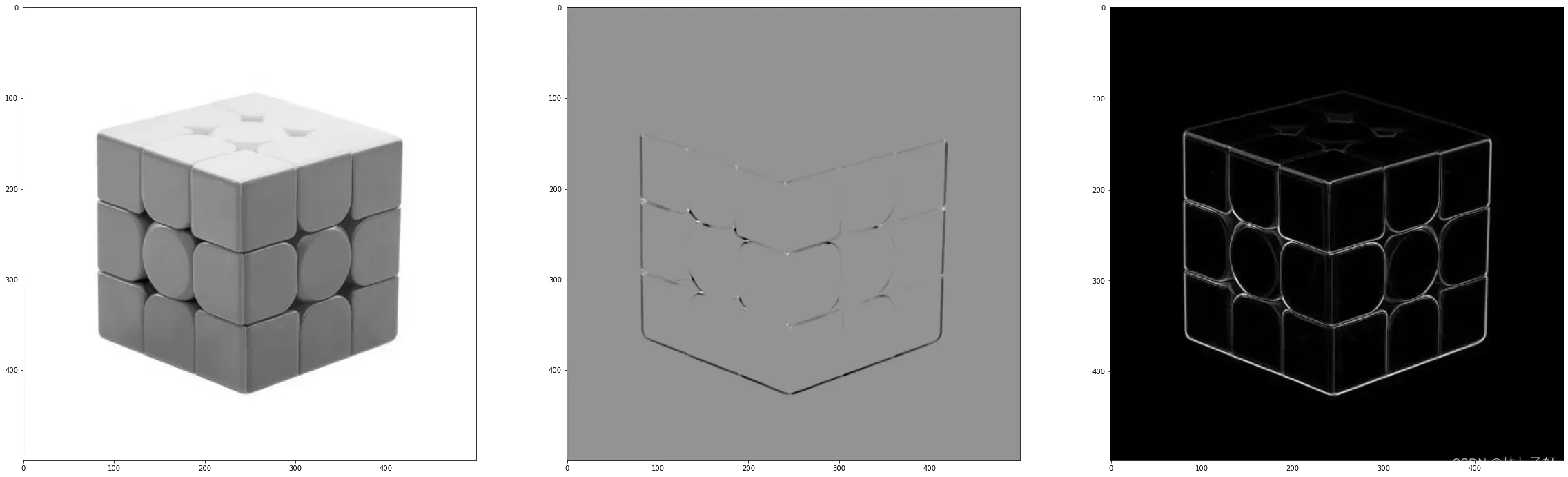
plt.figure(figsize=(40,40))
plt.subplot(131)
plt.imshow(magic_cube_gray,cmap ='gray')
plt.subplot(132)
plt.imshow(corners_Harris,cmap='gray')
plt.subplot(133)
plt.imshow(cube_G_L1,cmap='gray')
plt.show()
'''如下图所示，直接显示的检测效果并不理想，但sobel算子运算得到的边缘图十分明显
cube的上面灰度值与255较为接近，偏差不明显，之后使用threshold进行角点检测'''

'如下图所示，直接显示的检测效果并不理想，
cube的上面灰度值与255较为接近，偏差不明显，故而使用threshold'筛选数据

'''对该函数进行阈值处理，如果 G > threshold，表示该窗口对应一个角点特征.'''
threshold= 0.01*corners_Harris.max()
flag = corners_Harris > threshold


'''方法1，由np.where 直接找到 符合条件的array 下标'''
# where(condition, [x, y])
# x,y = np.where(flag) #返回tuple 返回了一个基于原本数据的地址索引 type() -> 2
x,y = np.where(flag)

corners_data1 = []
for i,j in zip(x,y):
    corners_data1.append(corners_Harris[i][j])
'''方法2，由 统计学习的数学运算方法传入一个由True，false组成的flag，
直接得到一个符合条件的一维数据'''
corners_data2 = corners_Harris[flag]


'''测试data_index 所指向的数据是否和corners_data所记录的符合的数据一致'''
corners_data1 == corners_data2
#数据比对均为True，说明由方法1和方法2获得的数据一样

array([ True,  True,  True,  True,  True,  True,  True,  True,  True,
        True,  True,  True,  True,  True,  True,  True,  True,  True,
        True,  True,  True,  True,  True,  True,  True,  True,  True,
        True,  True,  True,  True,  True,  True,  True,  True,  True,
        True,  True,  True,  True,  True,  True,  True,  True,  True,
        True,  True,  True,  True,  True,  True,  True,  True,  True,
        True,  True,  True,  True,  True,  True,  True,  True,  True,
        True,  True,  True,  True,  True,  True,  True,  True,  True,
        True,  True,  True,  True,  True,  True,  True,  True,  True,
        True,  True,  True,  True,  True,  True,  True,  True,  True,
        True,  True,  True,  True,  True,  True,  True,  True,  True,
        True,  True,  True,  True,  True,  True,  True,  True,  True,
        True,  True,  True,  True,  True,  True,  True,  True,  True,
        True,  True,  True,  True,  True,  True,  True,  True,  True,
        True,  True,  True,  True,  True,  True,  True,  True,  True,
        True,  True,  True,  True,  True,  True,  True,  True,  True,
        True,  True,  True,  True,  True,  True,  True,  True,  True,
        True,  True,  True,  True,  True,  True,  True,  True,  True,
        True,  True,  True,  True,  True,  True,  True,  True,  True,
        True,  True,  True,  True,  True])

'''对于方法2的解释说明'''
a = np.array([[1,2,3],[1,2,3]])
flag1 = np.array([[True,True,True],[False,True,False]])
b = a[flag1] #这种方法只是返回合格的数据，但并没有原始数据所在的下标，且形状为1维，适合label标签的选取分类

'''plot 绘制角点'''
plt.figure(figsize=(40,40))
plt.subplot(121)
plt.scatter(y,x,c = 'red')
plt.imshow(magic_cube_gray,cmap='gray')
plt.subplot(122)
plt.scatter(y,x,c = 'red')
plt.imshow(cube_G_L1,cmap='gray')
plt.show()
plt.savefig('figures/cube_Harris.png')

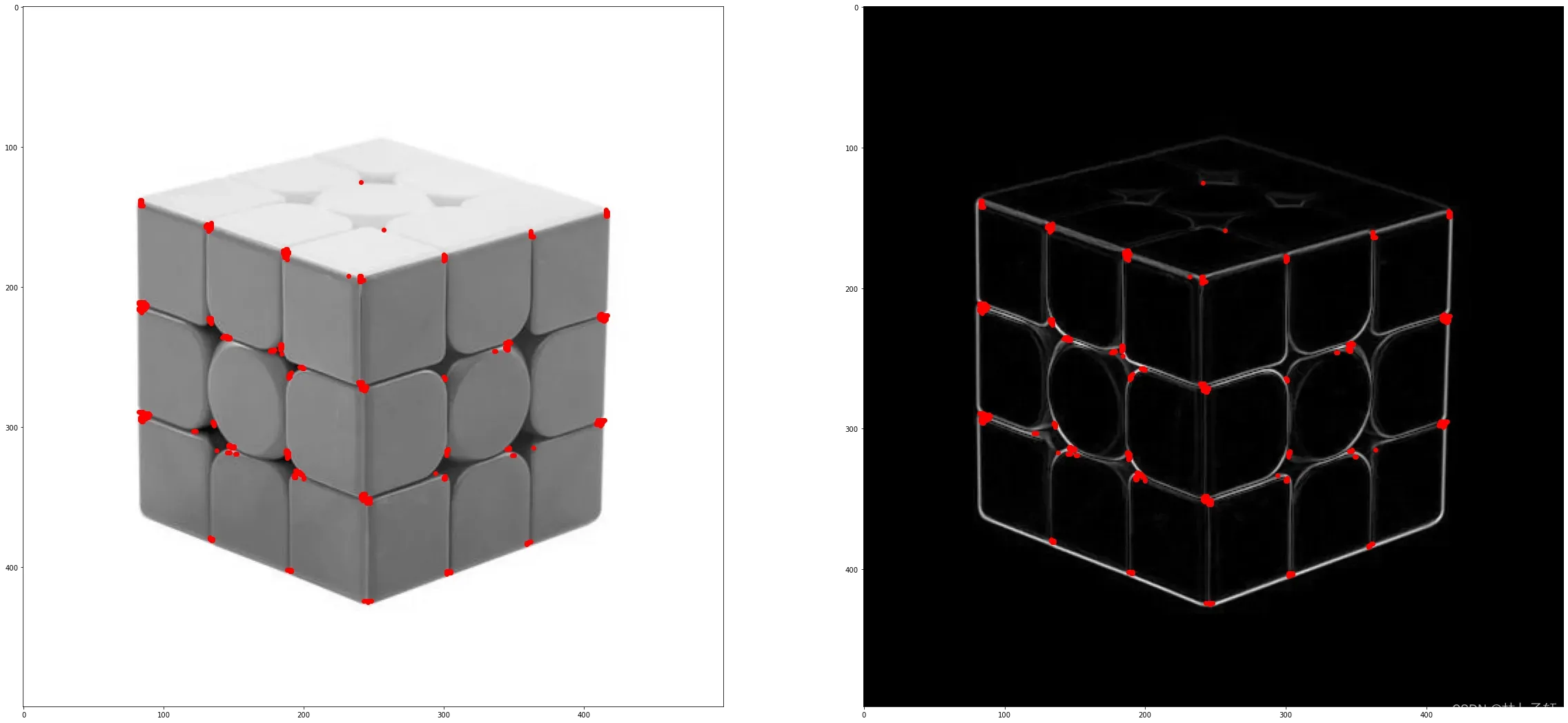
如上图所示,角点位置坐标全部标注为红色,数据在X,Y中保存对应的位置下标,实测所知,得到的数据x
,y转换后可以正常画图使用 即x,y = y,x

推荐文章
主成分分析，独立成分分析，+t-SNE 分布随机可视化降维的对比
线性回归预测波士顿房价
基于逻辑回归的虹膜分类
数据表示和特征工程
参考
机器学习 使用OpenCV、Python和scikit-learn进行智能图像处理(原书第2版)-(elib.cc) by (印)阿迪蒂亚·夏尔马(Aditya Sharma)(印)维什韦什·拉维·什里马利(Vishwesh Ravi Shrimali)(美)迈克尔·贝耶勒(Michael Beyeler)
Sobel算子，百度百科
角点检测Harris与Shi-Tomas