1. 实现SRN
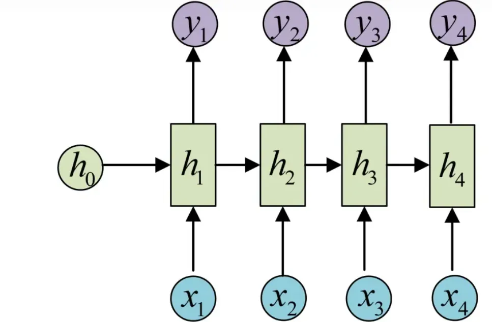
RNN【循环神经网络】通过使用带自反馈的神经元,能够处理任意长度的时序数据,如下图所示:
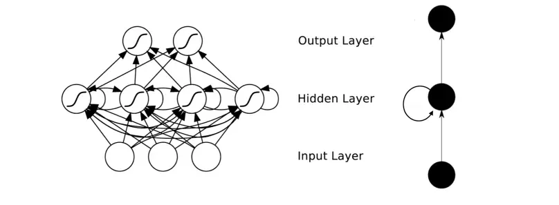
图来自【RNN及其简单Python代码示例_rnn python代码-CSDN博客】
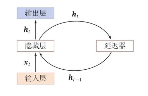
而SRN,也就是简单循环神经网络,只有一个隐藏层,如下图所示:
(1)使用Numpy

import numpy as np
inputs=np.array([[1.,1.],[1.,1.],[2.,2.]])
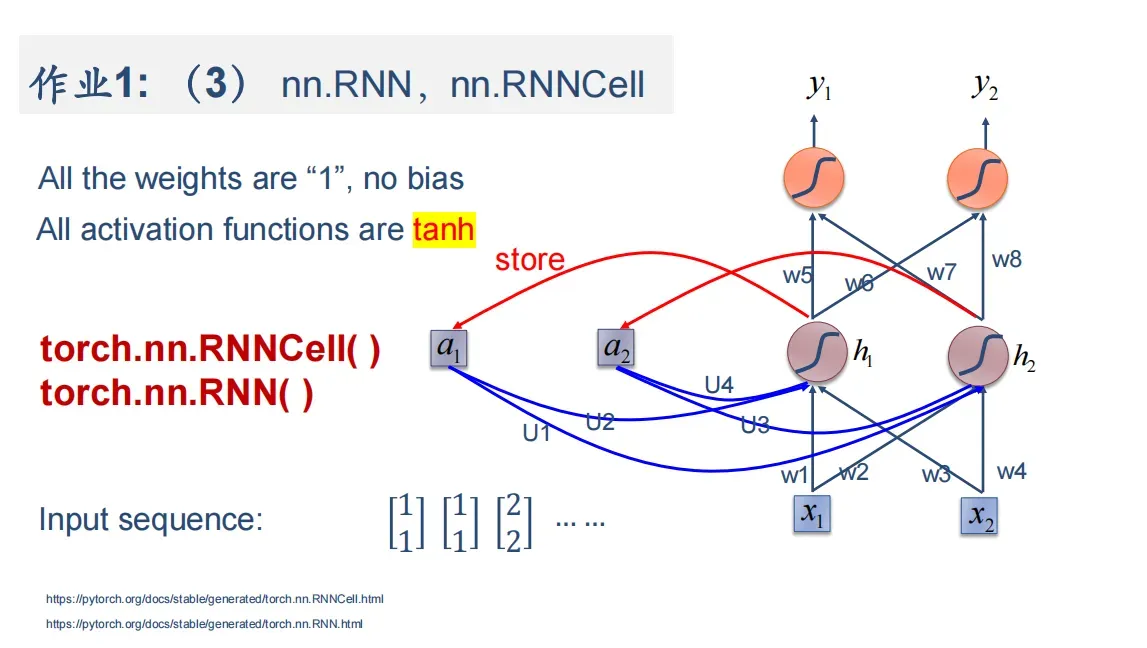
w1, w2, w3, w4, w5, w6, w7, w8 = 1., 1., 1., 1., 1., 1., 1., 1.
U1, U2, U3, U4 = 1., 1., 1., 1.
print('inputs is',inputs)
state_t=np.zeros(2,)
print('state_t is',state_t)
print('----------------')
#遍历输入的每一组x
for input_t in inputs:
print('inputs is',input_t)
print('state_t is',state_t)
#全连接【tanh(输入*线性权重)】+延迟器*状态权重
in_h1 = np.dot([w1, w3], input_t) + np.dot([U2, U4], state_t)
in_h2 = np.dot([w2, w4], input_t) + np.dot([U1, U3], state_t)
#更新延迟期
state_t=(in_h1, in_h2)
#全连接
output_y1 = np.dot([w5, w7], [in_h1, in_h2])
output_y2 = np.dot([w6, w8], [in_h1, in_h2])
print('output_y is',output_y1,output_y2)
print('--------------')
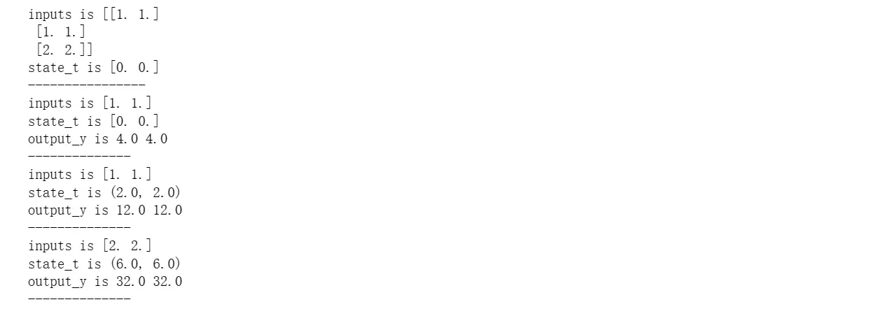
结果为:
(2)在1的基础上,增加激活函数tanh

import numpy as np

inputs=np.array([[1.,1.],[1.,1.],[2.,2.]])
w1, w2, w3, w4, w5, w6, w7, w8 = 1., 1., 1., 1., 1., 1., 1., 1.
U1, U2, U3, U4 = 1., 1., 1., 1.

print('inputs is',inputs)
state_t=np.zeros(2,)
print('state_t is',state_t)
print('----------------')

#增加激活函数

#遍历输入的每一组x
for input_t in inputs:
    print('inputs is',input_t)
    print('state_t is',state_t)

    #全连接【tanh(输入*线性权重)】+延迟器*状态权重
    x1=np.dot([w1,w3],input_t[0])
    x1 = np.tanh(x1)
    in_h1=x1+np.dot([U2,U4],state_t)
    x2=np.dot([w2, w4],input_t[1])
    x2 = np.tanh(x2)
    in_h2=x2+np.dot([U1,U3],state_t)

    #更新延迟期
    state_t=(in_h1, in_h2)

    #全连接
    output_y1=np.dot([w5,w7],[in_h1[0],in_h2[0]])
    output_y2=np.dot([w6,w8],[in_h1[1],in_h2[1]])
    print('output_y is',output_y1,output_y2)
    print('--------------')
结果为:

(3)使用nn.RNNCell实现
import torch
batch_size=1
input_size=2
seq_len=3#序列长度:[1.,1.],[1.,1.],[2.,2.]
hidden_size=2#隐藏层维度:[1.,1.]
output_size=2#输出层维度
#RNNCell
cell=torch.nn.RNNCell(input_size=input_size,hidden_size=hidden_size)
for name,params in cell.named_parameters():
if name.startswith("weight"):#权重设置【1或0】
torch.nn.init.ones_(params)
else:
torch.nn.init.zeros_(params)
#线性层
linear=torch.nn.Linear(hidden_size,output_size)
linear.weight.data=torch.Tensor([[1,1],[1,1]])
linear.bias.data=torch.Tensor([0,0])
#输入
seq=torch.Tensor([[[1, 1]],
[[1, 1]],
[[2, 2]]])
#隐藏层初始设置为0
hidden=torch.zeros(batch_size,hidden_size)
output=torch.zeros(batch_size,output_size)
#输出
for idx,inputs in enumerate(seq):
#用===划开
print('='*20,idx,'='*20)
print('Input:',inputs)
print('hidden:',hidden)
#求解循环网络单元
hidden=cell(inputs,hidden)
#全连接
output=linear(hidden)
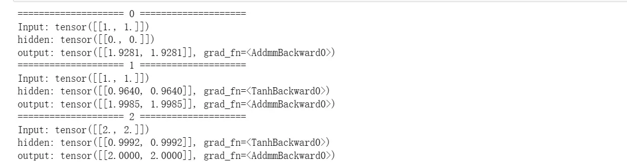
print('output:',output)结果为:
(4)使用nn.RNN实现
import torch

batch_size = 1
seq_len = 3
input_size = 2
hidden_size = 2
num_layers = 1#层数
output_size = 2

cell = torch.nn.RNN(input_size=input_size, hidden_size=hidden_size, num_layers=num_layers)
for name, param in cell.named_parameters():  # 初始化参数【1或0】
    if name.startswith("weight"):
        torch.nn.init.ones_(param)
    else:
        torch.nn.init.zeros_(param)

# 全连接【从隐藏层--输出】
liner = torch.nn.Linear(hidden_size, output_size)
liner.weight.data = torch.Tensor([[1, 1], [1, 1]])#线性层权重
liner.bias.data = torch.Tensor([0.0])#偏置

inputs = torch.Tensor([[[1, 1]],[[1, 1]],[[2, 2]]])
hidden = torch.zeros(num_layers, batch_size, hidden_size)
out, hidden = cell(inputs, hidden)#建立循环网络

print('Input :', inputs[0])
print('hidden:', 0, 0)
print('Output:', liner(out[0]))
print('--------------------------------------')
print('Input :', inputs[1])
print('hidden:', out[0])
print('Output:', liner(out[1]))
print('--------------------------------------')
print('Input :', inputs[2])
print('hidden:', out[1])
print('Output:', liner(out[2]))
输出为:

2. 实现“序列到序列”
观看视频,学习RNN原理,并实现视频P12中的教学案例
12.循环神经网络(基础篇)_哔哩哔哩_bilibili
(1)什么是RNN
RNN与与以前Linear线性层的区别:RNN的权重是共享的。
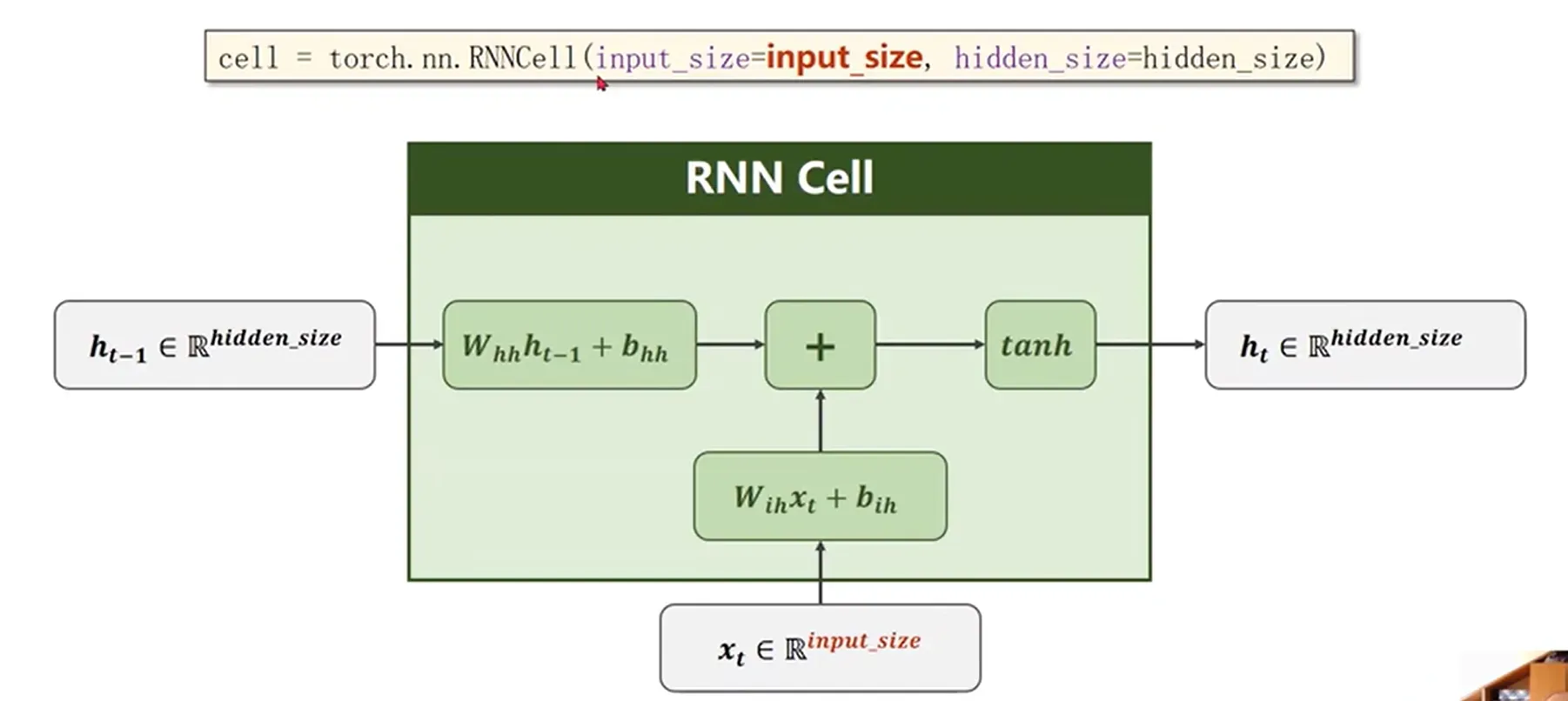
1)RNNCell
把RNNCell(下图中的一个单元)如下图,以循环的形式把序列送进去,依次算出隐藏层的过程就是循环神经网络。【本质上还是个线性层】
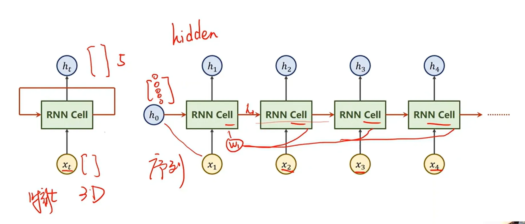
如下图所示,本次的输入=输入+上次的隐藏层,也就是:,本质上还是线性层。
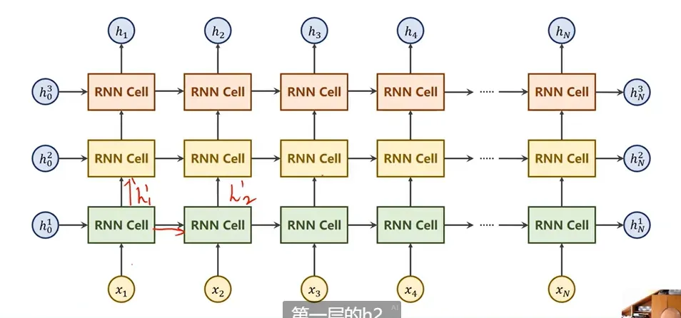
2)RNN
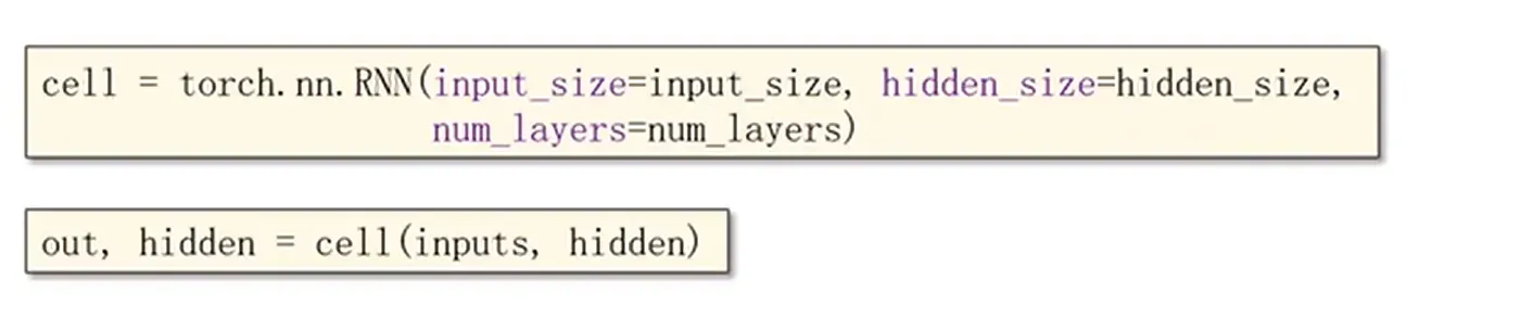 其中多了一层关于循环网络的层数num_layers【如下图所示】。
(2)input of shape & hidden of shape
1)RNNCell
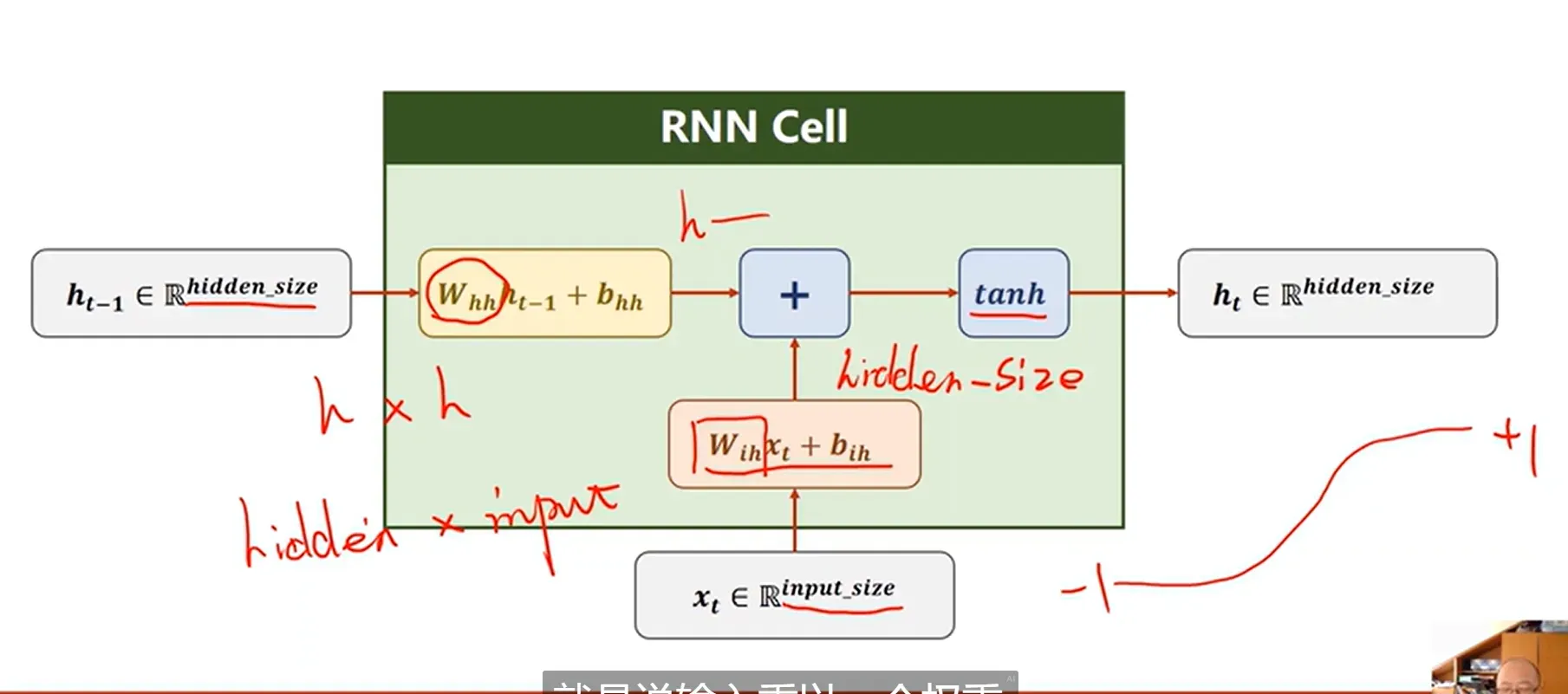
主要是输入的维度和隐藏的维度—-》就可以确定权重的维度和偏置的维度
 调用Cell时:输入input和hidden

在第4小节可以看到对RNNCell的总结,也就是按批量输入,上图可以看到维度情况。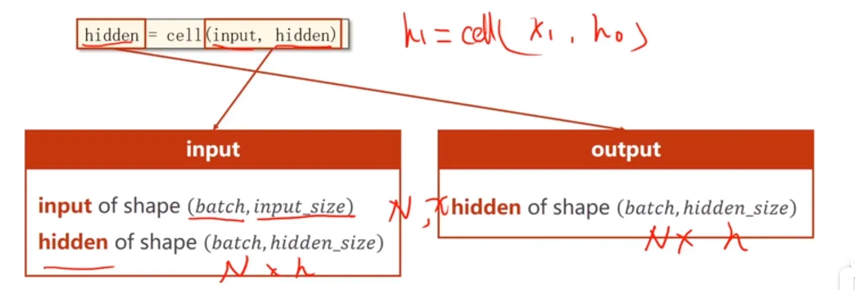
2)RNN
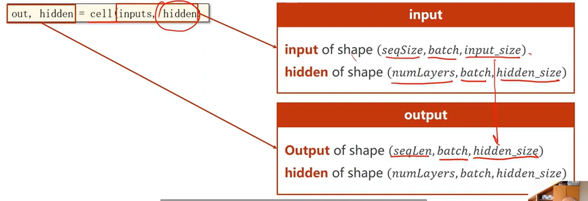
1)与2)图对比可以看到使用RNN与RNNCell的区别。
还可以变化:

(3)RNNCell如何使用?【例子】

import torch

batch_size=1 #批量大小
seq_len=3 #序列长度  x1,x2,x3
input_size=4 #输入是四维:竖着【0*4】【】【】
hidden_size=2 #隐藏层维度为2维:竖着【0*2】【】【】

#构造循环神经单元
cell=torch.nn.RNNCell(input_size=input_size,hidden_size=hidden_size)

#seq_len,btach,input
dataset=torch.randn(seq_len,batch_size,input_size)
hidden=torch.zeros(batch_size,hidden_size)

for idx,input in enumerate(dataset):
    print('='*20,idx,'='*20)
    print('Input_size:',input.shape)

    hidden=cell(input,hidden)

    print('outputs size:',hidden.shape)
    print(hidden)
结果为:
==================== 0 ====================
Input_size: torch.Size([1, 4])
outputs size: torch.Size([1, 2])
tensor([[-0.8622, -0.0829]], grad_fn=<TanhBackward0>)
==================== 1 ====================
Input_size: torch.Size([1, 4])
outputs size: torch.Size([1, 2])
tensor([[-0.8829,  0.4816]], grad_fn=<TanhBackward0>)
==================== 2 ====================
Input_size: torch.Size([1, 4])
outputs size: torch.Size([1, 2])
tensor([[-0.2461,  0.9268]], grad_fn=<TanhBackward0>)
(4)RNN如何使用?【例子】
import torch

batch_size=1
seq_len=3
input_size=4
hidden_size=2
num_layers=1#层数

cell=torch.nn.RNN(input_size=input_size,hidden_size=hidden_size,num_layers=num_layers)

#seq_Len,batch_size,input_size
inputs=torch.randn(seq_len,batch_size,input_size)
hidden=torch.zeros(num_layers,batch_size,hidden_size)

out,hidden=cell(inputs,hidden)

print('Output size:',out.shape)
print('Output size:',out)
print('Hidden size:',hidden.shape)
print('Hidden:',hidden)
结果为:
Output size: torch.Size([3, 1, 2])
Output size: tensor([[[-0.8859,  0.2043]],

        [[-0.6862,  0.5391]],

        [[-0.8006, -0.0733]]], grad_fn=<StackBackward0>)
Hidden size: torch.Size([1, 1, 2])
Hidden: tensor([[[-0.8006, -0.0733]]], grad_fn=<StackBackward0>)
(5)序列到序列的例子【‘h-e-l-l-o’—>’o-h-l-o-l’】
1)序列转化成数组
举个例子,比如说‘hello’这个序列,因为需要转换成数组形式,类似独热编码,如下图:

我们把从序列转化后的数组叫做独热向量。 其中input_size=4,seq_len=5
2) RNNCell举例
import torch
#参数
input_size = 4
hidden_size = 4  # 输出维度要与输入一致,才能在同一个表上查询
batch_size = 1

# Prepare Data
index2char = ['e', 'h', 'l', 'o']  # 字典
x_data = [1, 0, 2, 2, 3]  # hello
y_data = [3, 1, 2, 3, 2]  # 标签:ohlol
# one-hot向量:用来做查询【seq_len*input_size】
one_hot_lookup = [[1, 0, 0, 0],  # x_data参照one-hot向量得到对应序列
                  [0, 1, 0, 0],
                  [0, 0, 1, 0],
                  [0, 0, 0, 1]]

# 转化为独热向量,维度(seq, batch, input)
x_one_hot = [one_hot_lookup[x] for x in x_data]
#转为Tensor
inputs = torch.Tensor(x_one_hot).view(-1, batch_size, input_size)
# 每标签:计算交叉熵损失时不进行one-hot编码
labels = torch.LongTensor(y_data).view(-1, 1)

#Design Model
class Model(torch.nn.Module):
    def __init__(self, input_size, hidden_size, batch_size):  # 需要指定输入,隐层,批
        super(Model, self).__init__()
        #参数初始化
        self.batch_size = batch_size
        self.input_size = input_size
        self.hidden_size = hidden_size
        self.rnncell = torch.nn.RNNCell(input_size=self.input_size, hidden_size=hidden_size)

    def forward(self, input, hidden):
        #ht=Cell(xt,ht-1)
        hidden =self.rnncell(input, hidden)
        return hidden

    def init_hidden(self):  # 工具:生成初始的0----只有构造h0的需要
        return torch.zeros(self.batch_size, self.hidden_size)


net = Model(input_size, hidden_size, batch_size)

# 4.loss & optimizer
criterion = torch.nn.CrossEntropyLoss()
#改进的优化器Adam
optimizer = torch.optim.Adam(net.parameters(), lr=0.1)

# 5.Model Training
for epoch in range(15):
    #损失初始0
    loss = 0
    optimizer.zero_grad()
    hidden = net.init_hidden()  # 计算h0
    print('Predicted string:', end='')

    #其中inputs.shape=seq_len*batch_size*input_size
    for input, label in zip(inputs, labels):
        #input 遍历不同序列
        hidden = net(input, hidden)
        loss += criterion(hidden, label)  # 总损失需要构建计算图,不能取item()
        _, idx = hidden.max(dim=1)  # 取出概率最大的索引
        print(index2char[idx.item()], end='')
    loss.backward()#进行优化
    optimizer.step()
    print(',Epoch [%d / 15] loss:%.4f' % (epoch+1, loss.item()))
结果为:
Predicted string:lhhhh,Epoch [1 / 15] loss:7.6925
Predicted string:lhlhl,Epoch [2 / 15] loss:6.2360
Predicted string:lhlhl,Epoch [3 / 15] loss:5.1942
Predicted string:lhlhl,Epoch [4 / 15] loss:4.3271
Predicted string:ohlol,Epoch [5 / 15] loss:3.7150
Predicted string:ohlol,Epoch [6 / 15] loss:3.3898
Predicted string:ohlol,Epoch [7 / 15] loss:3.1891
Predicted string:ohlol,Epoch [8 / 15] loss:3.0256
Predicted string:ohlol,Epoch [9 / 15] loss:2.8745
Predicted string:ohlol,Epoch [10 / 15] loss:2.7311
Predicted string:ohlol,Epoch [11 / 15] loss:2.5962
Predicted string:ohlol,Epoch [12 / 15] loss:2.4769
Predicted string:ohlol,Epoch [13 / 15] loss:2.3775
Predicted string:ohlol,Epoch [14 / 15] loss:2.2932
Predicted string:ohlol,Epoch [15 / 15] loss:2.2205
3)RNN举例
import torch

# 参数
seq_len = 5
input_size = 4
hidden_size = 4
batch_size = 1

# Data Prepare
index2char = ['e', 'h', 'l', 'o']
x_data = [1, 0, 2, 2, 3]
y_data = [3, 1, 2, 3, 2]
one_hot_lookup = [[1, 0, 0, 0],
                  [0, 1, 0, 0],
                  [0, 0, 1, 0],
                  [0, 0, 0, 1]]
#独热向量
x_one_hot = [one_hot_lookup[x] for x in x_data]
inputs = torch.Tensor(x_one_hot).view(-1, batch_size, input_size)
labels = torch.LongTensor(y_data)

# Model Building
class Model(torch.nn.Module):
    def __init__(self, input_size, hidden_size, batch_size, num_layers=1):  # 【输入维度,隐层维度,批量,层数】
        #初始化
        super(Model, self).__init__()
        self.batch_size = batch_size
        self.input_size = input_size
        self.hidden_size = hidden_size
        self.num_layers = num_layers
        #调用RNN模型
        self.rnn = torch.nn.RNN(input_size=self.input_size, hidden_size=self.hidden_size, num_layers=self.num_layers)

    def forward(self, input):#h0
        hidden = torch.zeros(self.num_layers,
                             self.batch_size,
                             self.hidden_size)
        out, _ = self.rnn(input, hidden)  # out.shape=seq_len*batch*hidden_size
        return out.view(-1, self.hidden_size)  # 将输出的三维张量转换为二维张量,(seq_len*batch_size,hidden_size)

net = Model(input_size, hidden_size, batch_size)

#loss optimizer
criterion = torch.nn.CrossEntropyLoss()
optimizer = torch.optim.Adam(net.parameters(), lr=0.5)

# 5.Model Training
for epoch in range(15):
    #train steps
    optimizer.zero_grad()
    outputs = net(inputs)
    print(outputs.shape)
    loss = criterion(outputs, labels)
    loss.backward()
    optimizer.step()
    #输出
    _, idx = outputs.max(dim=1)
    idx = idx.data.numpy()
    print('Predicted string: ', ''.join([index2char[x] for x in idx]), end='')
    print(',Epoch [%d / 15] loss:%.4f' % (epoch+1, loss.item()))
结果为:
torch.Size([5, 4])
Predicted string:  lehhh,Epoch [1 / 15] loss:1.5116
torch.Size([5, 4])
Predicted string:  ohohh,Epoch [2 / 15] loss:1.2975
torch.Size([5, 4])
Predicted string:  oelhl,Epoch [3 / 15] loss:0.8748
torch.Size([5, 4])
Predicted string:  oelol,Epoch [4 / 15] loss:0.7066
torch.Size([5, 4])
Predicted string:  ohlol,Epoch [5 / 15] loss:0.5675
torch.Size([5, 4])
Predicted string:  ohlol,Epoch [6 / 15] loss:0.5582
torch.Size([5, 4])
Predicted string:  ohlol,Epoch [7 / 15] loss:0.5486
torch.Size([5, 4])
Predicted string:  ohlol,Epoch [8 / 15] loss:0.5294
torch.Size([5, 4])
Predicted string:  ohlol,Epoch [9 / 15] loss:0.4968
torch.Size([5, 4])
Predicted string:  ohlol,Epoch [10 / 15] loss:0.4797
torch.Size([5, 4])
Predicted string:  ohlol,Epoch [11 / 15] loss:0.4533
torch.Size([5, 4])
Predicted string:  ohlol,Epoch [12 / 15] loss:0.4375
torch.Size([5, 4])
Predicted string:  ohlol,Epoch [13 / 15] loss:0.4258
torch.Size([5, 4])
Predicted string:  ohlol,Epoch [14 / 15] loss:0.4122
torch.Size([5, 4])
Predicted string:  ohlol,Epoch [15 / 15] loss:0.3907
比较2)与3)的结果:可以发现,使用RNN模型比调用RNNCell模型更简单,并且效果更好【损失更低】
4)独热码特点

也就是说:
词级的维度太高
向量过于稀疏
硬编码,不是通过学习出来的
5)Embedding【数据降维】
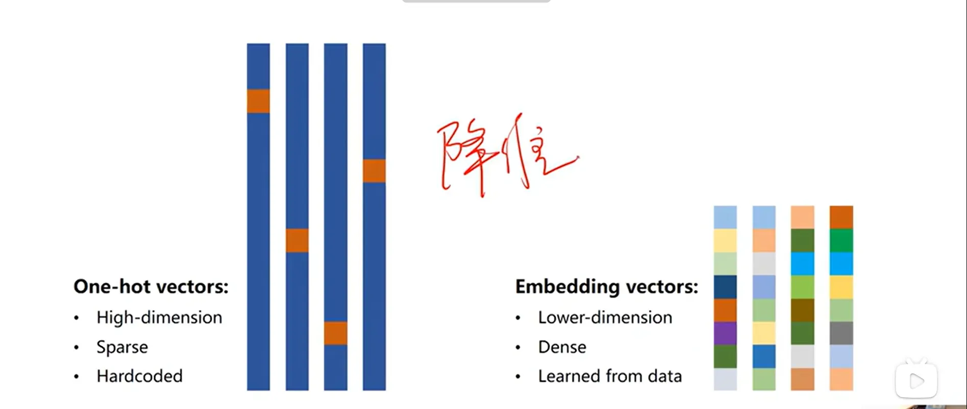
降维方式: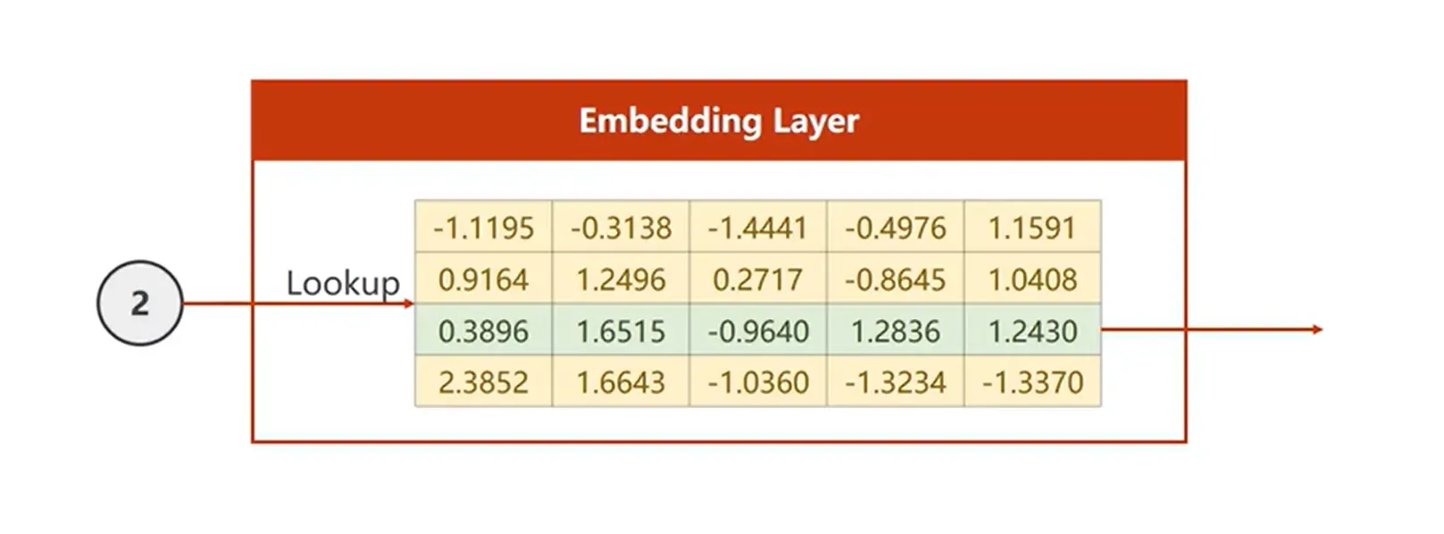
由上图所示:输入为2,也就是要查找第二个字符,在列表中找到第二行直接输出。
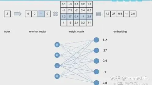
或者如下图所示更加直观【图来自Embedding技术的本质(图解) – 知乎 (zhihu.com)】:
其中有关它的参数如下:【图来自神经网络中embedding层作用——本质就是word2vec,数据降维,同时可以很方便计算同义词(各个word之间的距离),底层实现是2-gram(词频)+神经网络_51CTO博客_embedding 神经网络】
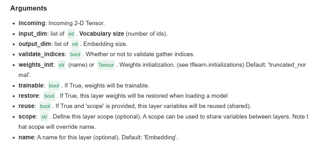
其中比较重要的是输入和输出参数 :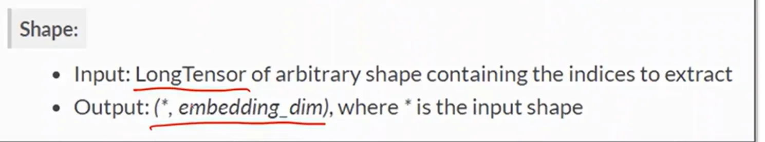
输入变三维seq*batch_size*embedding
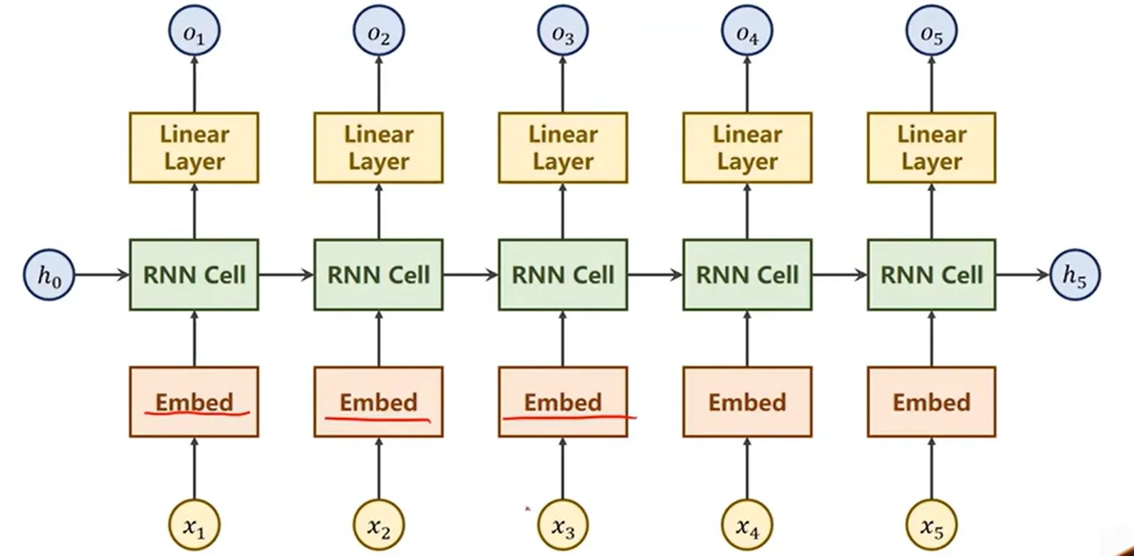
那么加入嵌入层后的循环神经网络是:
6)加入embedding的例子
import torch
# 参数
num_class = 4
input_size = 4
hidden_size = 8
embedding_size = 10#嵌入层
num_layers = 2
batch_size = 1
seq_len = 5

# Data prepare
index2char = ['e', 'h', 'l', 'o']
x_data = [[1, 0, 2, 2, 3]]  # (batch_size, seq_len):hello
y_data = [3, 1, 2, 3, 2]  # (batch_size * seq_len) :ohlol

inputs = torch.LongTensor(x_data)  # (batch_size, seq_len)
labels = torch.LongTensor(y_data)  # (batch_size * seq_len)

#Model Building
class Model(torch.nn.Module):
    def __init__(self):
        super(Model, self).__init__()
        self.emb = torch.nn.Embedding(num_class, embedding_size)
        self.rnn = torch.nn.RNN(input_size=embedding_size, hidden_size=hidden_size, num_layers=num_layers,
                                batch_first=True)
        self.fc = torch.nn.Linear(hidden_size, num_class)

    def forward(self, x):
        hidden = torch.zeros(num_layers, x.size(0), hidden_size)  # (num_layers, batch_size, hidden_size)
        x = self.emb(x)  # 返回(batch_size, seq_len, embedding_size)三维
        x, _ = self.rnn(x, hidden)  # 返回(batch_size, seq_len, hidden_size)
        x = self.fc(x)  # 返回(batch_size, seq_len, num_class)
        return x.view(-1, num_class)  # (batch_size * seq_len, num_class)


net = Model()

# loss optimizer
criterion = torch.nn.CrossEntropyLoss()
optimizer = torch.optim.Adam(net.parameters(), lr=0.05)

# Data training
for epoch in range(15):
    optimizer.zero_grad()
    outputs = net(inputs)
    loss = criterion(outputs, labels)
    loss.backward()
    optimizer.step()

    _, idx = outputs.max(dim=1)
    idx = idx.data.numpy()
    print('Predicted string: ', ''.join([index2char[x] for x in idx]), end='')
    print(', Epoch [%d/15] loss: %.4f' % (epoch + 1, loss.item()))
结果为:
Predicted string:  oolll, Epoch [1/15] loss: 1.3046
Predicted string:  oolll, Epoch [2/15] loss: 1.0554
Predicted string:  oolll, Epoch [3/15] loss: 0.8950
Predicted string:  ohlll, Epoch [4/15] loss: 0.7359
Predicted string:  ohlll, Epoch [5/15] loss: 0.5649
Predicted string:  ohlol, Epoch [6/15] loss: 0.3846
Predicted string:  ohlol, Epoch [7/15] loss: 0.2786
Predicted string:  ohlol, Epoch [8/15] loss: 0.1900
Predicted string:  ohlol, Epoch [9/15] loss: 0.1268
Predicted string:  ohlol, Epoch [10/15] loss: 0.0829
Predicted string:  ohlol, Epoch [11/15] loss: 0.0530
Predicted string:  ohlol, Epoch [12/15] loss: 0.0350
Predicted string:  ohlol, Epoch [13/15] loss: 0.0251
Predicted string:  ohlol, Epoch [14/15] loss: 0.0188
Predicted string:  ohlol, Epoch [15/15] loss: 0.0142
可以看到,加入嵌入层的循环神经网络训练出来的效果最好,loss最低。
以上内容未标注的图都是来自【12.循环神经网络(基础篇)_哔哩哔哩_bilibili】
3. “编码器-解码器”的简单实现
seq2seq的PyTorch实现_哔哩哔哩_bilibili
Seq2Seq的PyTorch实现 – mathor (wmathor.com)
(1)什么是解码器、译码器?
定义:
- 编码器:将文本表示成向量【编码器部分使用循环神经网络(RNN或者卷积神经网络(CNN)来将输入序列编码成一个固定长度的向量表示。这个向量包含了输入序列的重要特征信息。】
- 解码器:向量表示成输出【解码器部分使用循环神经网络(RNN)来将编码器输出的向量解码成目标序列。解码器通过学习来生成与目标序列相匹配的输出。】
使用CNN构造序列模型参考论文:Attention Is All You Need, Convolutional Sequence to Sequence Learning 。
内容参考【编码器和解码器 – 简书 (jianshu.com)】
编码器-解码器(encoder-decoder)架构:为了处理这种类型的输入和输出, 我们可以设计一个包含两个主要组件的架构: 第一个组件是一个编码器: 它接受一个长度可变的序列作为输入, 并将其转换为具有固定形状的编码状态。 第二个组件是解码器: 它将固定形状的编码状态映射到长度可变的序列。 这被称为编码器-解码器架构, 如图所示。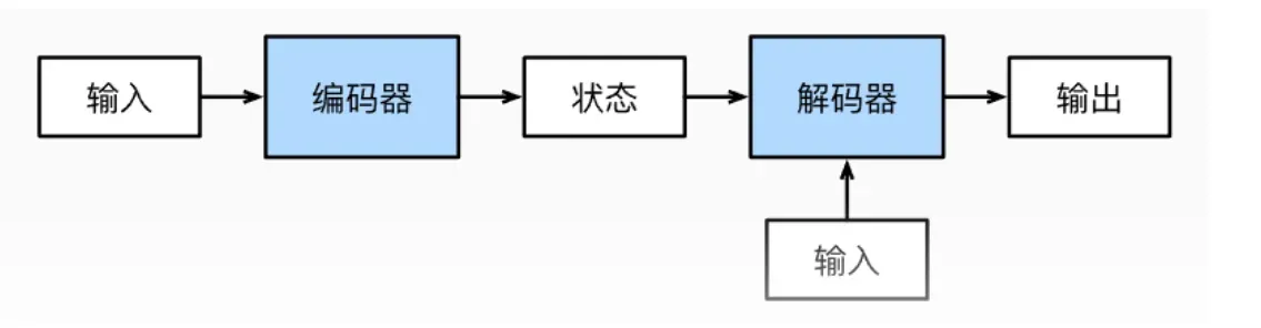
图文参考【编码器和解码器_enc解码-CSDN博客】
也就是说,一个模型可以被分为两块:
- 编码器处理输入
- 解码器生成输出
(2)实现
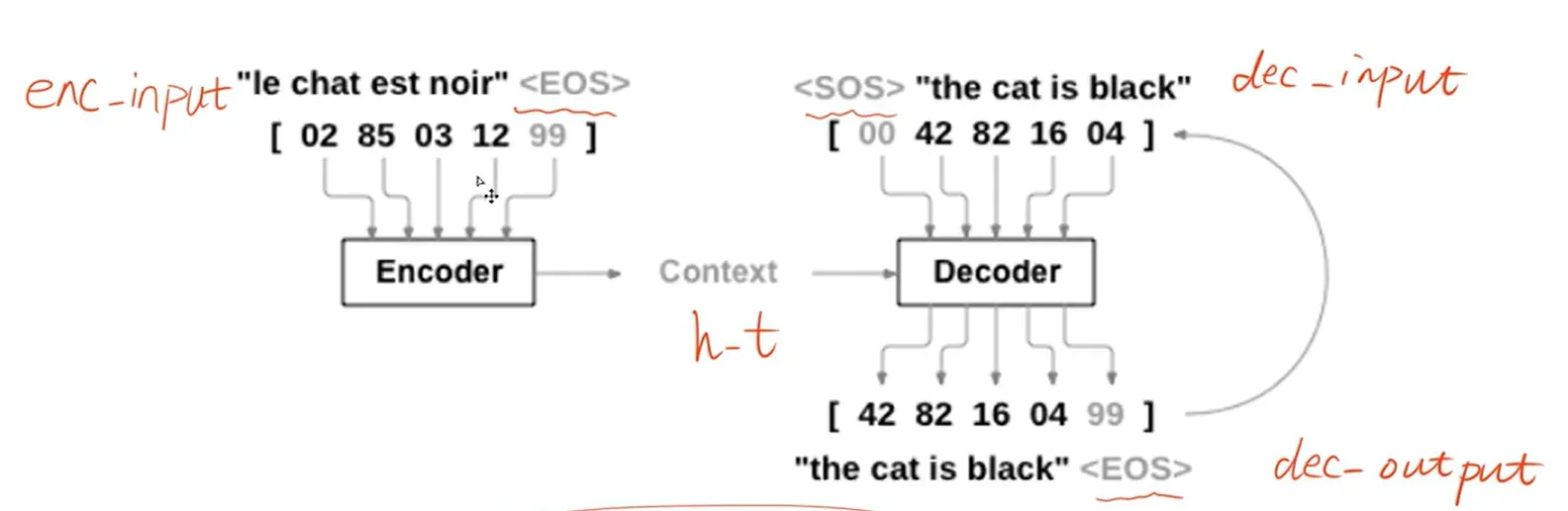
如下图所示,依次是:编码器输入–>上下文–>译码器输入–>译码器输出
# code by Tae Hwan Jung(Jeff Jung) @graykode, modify by wmathor
import torch
import numpy as np
import torch.nn as nn
import torch.utils.data as Data

device = torch.device('cuda' if torch.cuda.is_available() else 'cpu')
# S: Symbol that shows starting of decoding input:开始
# E: Symbol that shows starting of decoding output:结束标志
# ?: Symbol that will fill in blank sequence if current batch data size is short than n_step:类似填充

letter = [c for c in 'SE?abcdefghijklmnopqrstuvwxyz']
letter2idx = {n: i for i, n in enumerate(letter)}#letter转索引【字典】

seq_data = [['man', 'women'], ['black', 'white'], ['king', 'queen'], ['girl', 'boy'], ['up', 'down'], ['high', 'low']]

# Seq2Seq Parameter【参数】
n_step = max([max(len(i), len(j)) for i, j in seq_data])  # n_step=max_len(=5)
n_hidden = 128#隐藏状态的维度
n_class = len(letter2idx)  #分类
batch_size = 3


def make_data(seq_data):
    #与图中的对应
    enc_input_all, dec_input_all, dec_output_all = [], [], []

    #使用?补齐一组
    for seq in seq_data:
        for i in range(2):#一组两个
            seq[i] = seq[i] + '?' * (n_step - len(seq[i]))  # 举例:'man??'与'women'等长

        enc_input = [letter2idx[n] for n in (seq[0] + 'E')]  # ['m','a','n','?','?','E']
        dec_input = [letter2idx[n] for n in ('S' + seq[1])]  # ['S','w','o','m','e','n']
        dec_output = [letter2idx[n] for n in (seq[1] + 'E')]  # ['w','o','m','e','n','E']

        enc_input_all.append(np.eye(n_class)[enc_input])
        dec_input_all.append(np.eye(n_class)[dec_input])
        dec_output_all.append(dec_output)  # 不需要 one-hot 表示

    # 转成张量
    return torch.Tensor(enc_input_all), torch.Tensor(dec_input_all), torch.LongTensor(dec_output_all)


'''
对应维度:6个样本
enc_input_all: [6, n_step+1 (because of 'E'), n_class]
dec_input_all: [6, n_step+1 (because of 'S'), n_class]
dec_output_all: [6, n_step+1 (because of 'E')]
'''

#得到encoding、decoding【in/out】
enc_input_all, dec_input_all, dec_output_all = make_data(seq_data)

#保存编码器输入、解码器输入和解码器输出的数据
class TranslateDataSet(Data.Dataset):
    def __init__(self, enc_input_all, dec_input_all, dec_output_all):
        self.enc_input_all = enc_input_all
        self.dec_input_all = dec_input_all
        self.dec_output_all = dec_output_all

    def __len__(self):  # return dataset size
        return len(self.enc_input_all)

    def __getitem__(self, idx):#索引
        return self.enc_input_all[idx], self.dec_input_all[idx], self.dec_output_all[idx]

#数据加载
loader = Data.DataLoader(TranslateDataSet(enc_input_all, dec_input_all, dec_output_all), batch_size, True)


# 建立模型
class Seq2Seq(nn.Module):
    def __init__(self):
        super(Seq2Seq, self).__init__()
        #调用RNN
        self.encoder = nn.RNN(input_size=n_class, hidden_size=n_hidden, dropout=0.5)  # encoder
        self.decoder = nn.RNN(input_size=n_class, hidden_size=n_hidden, dropout=0.5)  # decoder
        #全连接
        self.fc = nn.Linear(n_hidden, n_class)

    def forward(self, enc_input, enc_hidden, dec_input):
        # enc_input(=input_batch): [batch_size, n_step+1, n_class]
        # dec_input(=output_batch): [batch_size, n_step+1, n_class]
        enc_input = enc_input.transpose(0, 1)  # enc_input: [n_step+1, batch_size, n_class]
        dec_input = dec_input.transpose(0, 1)  # dec_input: [n_step+1, batch_size, n_class]

        # h_t : [num_layers(=1) * num_directions(=1), batch_size, n_hidden]
        _, h_t = self.encoder(enc_input, enc_hidden)
        # outputs : [n_step+1, batch_size, num_directions(=1) * n_hidden(=128)]
        outputs, _ = self.decoder(dec_input, h_t)

        model = self.fc(outputs)  # model : [n_step+1, batch_size, n_class]
        return model


model = Seq2Seq().to(device)
#loss/optimizet\r
criterion = nn.CrossEntropyLoss().to(device)
optimizer = torch.optim.Adam(model.parameters(), lr=0.001)

#训练模型
for epoch in range(5000):
    for enc_input_batch, dec_input_batch, dec_output_batch in loader:
        # 隐藏层形状 [num_layers * num_directions, batch_size, n_hidden]
        h_0 = torch.zeros(1, batch_size, n_hidden).to(device)
        # enc_input_batch : [batch_size, n_step+1, n_class]
        # dec_intput_batch : [batch_size, n_step+1, n_class]
        # dec_output_batch : [batch_size, n_step+1], not one-hot
        (enc_input_batch, dec_intput_batch, dec_output_batch) = (enc_input_batch.to(device), dec_input_batch.to(device), dec_output_batch.to(device))

        # pred : [n_step+1, batch_size, n_class]------>[batch_size, n_step+1(=6), n_class]
        pred = model(enc_input_batch, h_0, dec_intput_batch)
        pred = pred.transpose(0, 1)
        loss = 0
        for i in range(len(dec_output_batch)):
            # pred[i] : [n_step+1, n_class]
            # dec_output_batch[i] : [n_step+1]
            loss += criterion(pred[i], dec_output_batch[i])
        if (epoch + 1) % 1000 == 0:
            print('Epoch:', '%04d' % (epoch + 1), 'cost =', '{:.6f}'.format(loss))

        optimizer.zero_grad()
        loss.backward()
        optimizer.step()


# 模型测试
def translate(word):
    enc_input, dec_input, _ = make_data([[word, '?' * n_step]])
    enc_input, dec_input = enc_input.to(device), dec_input.to(device)
    # make hidden shape [num_layers * num_directions, batch_size, n_hidden]
    hidden = torch.zeros(1, 1, n_hidden).to(device)
    output = model(enc_input, hidden, dec_input)
    # output : [n_step+1, batch_size, n_class]

    predict = output.data.max(2, keepdim=True)[1]  # select n_class dimension
    decoded = [letter[i] for i in predict]
    translated = ''.join(decoded[:decoded.index('E')])

    return translated.replace('?', '')


print('test')
print('man ->', translate('man'))
print('mans ->', translate('mans'))
print('king ->', translate('king'))
print('black ->', translate('black'))
print('up ->', translate('up'))
得到的结果为:
Epoch: 1000 cost = 0.002266
Epoch: 1000 cost = 0.002082
Epoch: 2000 cost = 0.000451
Epoch: 2000 cost = 0.000473
Epoch: 3000 cost = 0.000145
Epoch: 3000 cost = 0.000138
Epoch: 4000 cost = 0.000049
Epoch: 4000 cost = 0.000048
Epoch: 5000 cost = 0.000017
Epoch: 5000 cost = 0.000017
test
man -> women
mans -> women
king -> queen
black -> white
up -> down
4.简单总结nn.RNNCell、nn.RNN
(1)nn.package
在介绍这两个建立循环网络的重要因素之前,先介绍一下nn package:
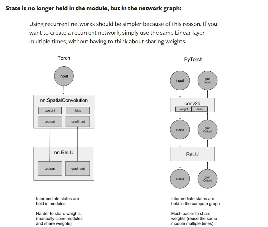
也就是使用nn包时:状态不再保存在模块中,而是保存在网络图中 ,使用循环网络更加简单速度更快。
Simplified debugging:
Debugging is intuitive using Python’s pdb debugger, and the debugger and stack traces stop at exactly where an error occurred. What you see is what you get.
调试代码也会变得简单。
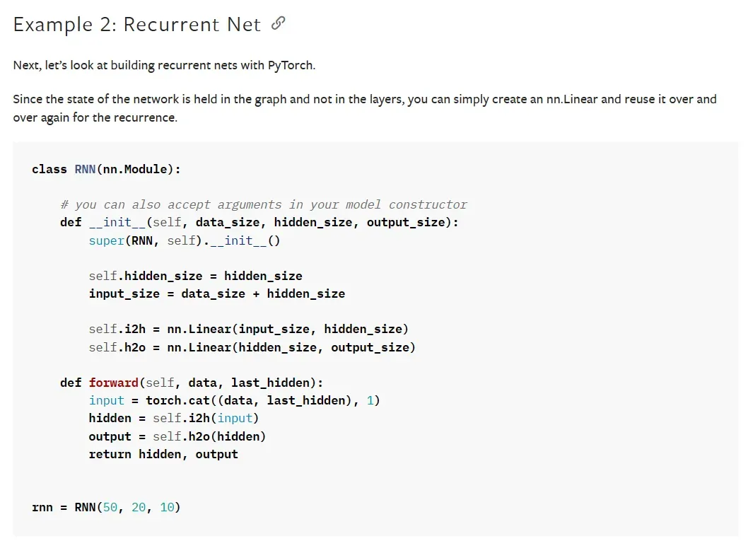
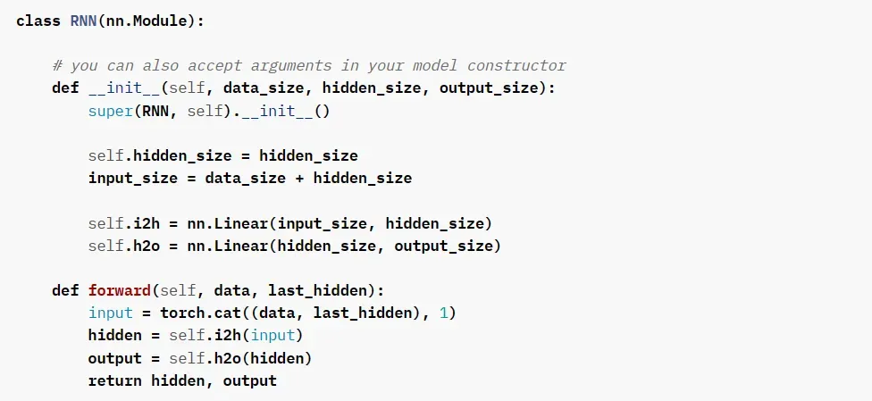
由于前边可以知道:网络的状态保存到图中,建立循环神经网络可以简单地创建一个 nn,线性层可以重复调试使用。
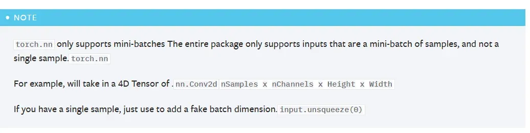
其中需要注意的是:torch.nn只支持小批量样本的输入 ,不支持单个样本输入。
参考nn package — PyTorch 教程 2.1.1+cu121 文档
(2)nn.RNNCell & nn.RNN
这一部分在第2小节中已经详细介绍过了【聊点别的】
1)调用类的主要内容
nn.RNNCell类:没有找到
nn.RNN类:
2)两者的区别
从我写的第2小节中的(3)与(4),可以看到RNN能够一次性的处理整个序列,而RNNCell只能处理序列中一个时间点的数据【RNN循环比RNNCell少一层】
其实也可以推断出:RNN更容易封装使用,RNNCell比RNN更具灵活性。
5.谈一谈对“序列”、“序列到序列”的理解
(1)什么是序列
序列的定义:在深度学习中一般为带有时间先后顺序(拥有逻辑结构)的一段具有连续关系的数据(文本,语音等等),或者是生活中有位置,顺序的固定序列信息。
内容参考【理解深度学习中的序列(sequence)以及RNN,CNN介绍_cnn序列-CSDN博客】
在前边的例子中应用的序列是单词。
(2)什么是序列到序列
前边解码器–译码器已经详细介绍了。
seq2seq是一种由双向RNN组成的encoder-decoder神经网络结构,从而满足输入输出序列长度不相同的情况,实现一个序列到另一个序列之间的转换。

序列到序列往往具有以下两个特点:
1. 输入输出时不定长的。比如说想要构建一个聊天机器人,你的对话和他的回复长度都是不定的。
2. 输入输出元素之间是具有顺序关系的。不同的顺序,得到的结果应该是不同的,比如“不开心”和“开心不”这两个短语的意思是不同的。
内容参考【序列到序列模型,了解一下 – 知乎 (zhihu.com)】
6.总结本周理论课和作业,写心得体会
主要学习了什么是RNN,以及RNN的两种实现方式【RNN与RNNCell】,这两种实现方式有什么差异【前文已经详细介绍了,这边就不重复了】
感悟比较深的就是序列到序列:首先把一个序列按照独热向量转成数组,然后将数组作为输入送到RNN模型中,得到输出。再深入一点,就是解码器到译码器的主要工作。
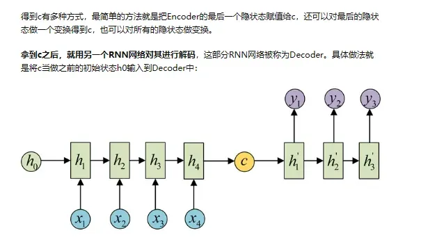
然后这里参考了【完全图解RNN、RNN变体、Seq2Seq、Attention机制 – 知乎 (zhihu.com)】进行扩展【最后搜到这个,感觉很有用!】:
1.序列到序列等长【同步】:
2.序列到类别

3.图像/类别到序列

4.序列到序列不等长【异步】
就是我们前文提到的seq2seq:
作业参考【【23-24 秋学期】NNDL 作业9 RNN – SRN-CSDN博客】
文章出处登录后可见!