机器学习之逻辑回归(Logit模型）实现—基于R语言（附完整代码）

大家好，我是带我去滑雪！

本期使用R包 ElemStatLearn 的南非心脏病数据 SAheart 进行逻辑回归。其中，响应变量为chd（是否有冠心病，即coronary heart disease）。特征向量包括sbp（收缩压，systolic blood pressure）、tobacco（累计抽烟量）、ldl（低密度脂蛋白胆固醇，即low density lipoprotein cholesterol）、因子变量famhist（是否有家族心脏病史）、typea（A型行为，即type-A behavior）、alcohol（当前饮酒量）、age（发病时年龄），以及两个关于肥胖程度的数值型度量adiposity与obesity。该案例来自陈强编著的《机器学习及R运用》第5.1节课后习题。

需要完成的工作有如下：
（1）将响应变量 cha 设为因子变量，并计算样本中有冠心病的比例；
（2）使用set. seed (1)，预留 100 个观测值作为测试集；
（3）使用训练集，将chd 对其余变量进行逻辑回归；
（4）计算此逻辑回归的准 $gif.latex?R%5E%7B2%7D$ ；
（5）计算平均边际效应AME，并画图展示；
（6）在测试集中进行预测，计算准确率、错误率、灵敏度、特异度与召回率；
（7）画ROC 曲线；
（8）计算 AUC:
（9）计算 kappa 值。

（0）加载包

首先尝试最常用的先安装包再加载数据集：

> install.packages(ElemStatLearn)
Error in install.packages : object ‘ElemStatLearn’ not found

结果显示：“Error in install.packages : object ‘ElemStatLearn’ not found”，所以采用这种方法安装ElemStatLearn包不行，正确的做法如下，使用“str()”查看数据结构：

>packageurl <- “https://cran.r-project.org/src/contrib/Archive/ElemStatLearn/ElemStatLearn_2015.6.26.tar.gz”
>install.packages(packageurl, repos=NULL, type=”source”)
>library(ElemStatLearn)
>str(SAheart)
‘data.frame’: 462 obs. of 10 variables:
$ sbp : int 160 144 118 170 134 132 142 114 114 132 …
$ tobacco : num 12 0.01 0.08 7.5 13.6 6.2 4.05 4.08 0 0 …
$ ldl : num 5.73 4.41 3.48 6.41 3.5 6.47 3.38 4.59 3.83 5.8 …
$ adiposity : num 23.1 28.6 32.3 38 27.8 …
$ famhist : Factor w/ 2 levels “Absent”,”Present”: 2 1 2 2 2 2 1 2 2 2 …
$ typea : int 49 55 52 51 60 62 59 62 49 69 …
$ obesity : num 25.3 28.9 29.1 32 26 …
$ alcohol : num 97.2 2.06 3.81 24.26 57.34 …
$ age : int 52 63 46 58 49 45 38 58 29 53 …
$ chd : int 1 1 0 1 1 0 0 1 0 1 …

（1）将响应变量 cha 设为因子变量，并计算样本中有冠心病的比例

> SAheart$chd=factor(SAheart$chd,levels = c(“1″,”0”),labels=c(“Have”,”Don’t have”))
> options(digits = 4)
> prop.table(table(SAheart$chd))
Have Don’t have
0.3463 0.6536

结果显示，样本中有冠心病的比例为34.63%，没有冠心病的比例为65.36%，其中“options(digits = 4)”表示保留小数点后四位数字。

（2）使用set. seed (1)，预留 100 个观测值作为测试集

> set.seed(1)
> train_index=sample(462,362)
> train=SAheart[train_index,]
> test=SAheart[-train_index,]
> str(train)
‘data.frame’: 362 obs. of 10 variables:
$ sbp : int 140 110 134 176 132 136 150 150 128 174 …
$ tobacco : num 8.6 12.2 8.8 0 12 …
$ ldl : num 3.9 4.99 7.41 3.14 4.51 7.84 6.4 5.04 2.43 6.57 …
$ adiposity: num 32.2 28.6 26.8 31 21.9 …
$ famhist : Factor w/ 2 levels “Absent”,”Present”: 2 1 1 2 1 2 1 2 2 2 …
$ typea : int 52 44 35 45 61 58 53 60 63 50 …
$ obesity : num 28.5 27.1 29.4 30.2 26.1 …
$ alcohol : num 11.11 21.6 29.52 4.63 64.8 …
$ age : int 64 55 60 45 46 45 63 45 17 64 …
$ chd : Factor w/ 2 levels “Have”,”Don’t have”: 1 1 1 2 1 1 2 2 2 1 …

（3）使用训练集，将chd 对其余变量进行逻辑回归

> options(digits=4)
> fit=glm(chd~.,data=train,family=binomial)
> summary(fit)
Call:
glm(formula = chd ~ ., family = binomial, data = train)
Deviance Residuals:
Min 1Q Median 3Q Max
-2.446 -0.871 0.456 0.786 1.887
Coefficients:
Estimate Std. Error z value Pr(>|z|)
(Intercept)   4.801815 1.464569 3.28 0.00104 **
sbp   -0.001488 0.006739 -0.22 0.82528
tobacco    -0.101163 0.029964 -3.38    0.00073 ***
ldl -0.181278 0.068809 -2.63 0.00843 **
adiposity -0.019735 0.032331 -0.61 0.54159
famhistPresent -0.801410 0.259376 -3.09    0.00200 **
typea -0.033687 0.013850 -2.43 0.01501 *
obesity 0.072542 0.048936 1.48 0.13824
alcohol -0.000867 0.005118 -0.17 0.86540
age -0.041313 0.013358 -3.09 0.00198 **
—
Signif. codes: 0 ‘***’ 0.001 ‘**’ 0.01 ‘*’ 0.05 ‘.’ 0.1 ‘ ’ 1
(Dispersion parameter for binomial family taken to be 1)
Null deviance: 465.32 on 361 degrees of freedom
Residual deviance: 369.50 on 352 degrees of freedom
AIC: 389.5
Number of Fisher Scoring iterations: 5

结果显示，经过5次“Fisher得分迭代”得到估计结果，其中，零偏离度（只有常数项模型的残差平方和）为465.32，而残差偏离度（完整模型的残差平方和）为369.50。

（4）计算此逻辑回归的准 $gif.latex?R%5E%7B2%7D$

> (fit$null.deviance-fit$deviance)/fit$null.deviance
[1] 0.2059

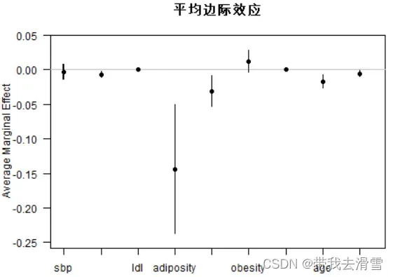
（5）计算平均边际效应AME，并画图展示

>install.packages(“margins”)
> library(margins)
> effects=margins(fit)
> summary(effects)
factor AME SE z p lower upper
adiposity -0.0033 0.0055 -0.6116 0.5408 -0.0141 0.0074
age -0.0070 0.0022 -3.2198 0.0013 -0.0113 -0.0027
alcohol -0.0001 0.0009 -0.1695 0.8654 -0.0018 0.0016
famhistPresent -0.1436 0.0473 -3.0344 0.0024 -0.2363 -0.0508
ldl -0.0307 0.0113 -2.7307 0.0063 -0.0528 -0.0087
obesity 0.0123 0.0082 1.5007 0.1334 -0.0038 0.0284
sbp -0.0003 0.0011 -0.2208 0.8252 -0.0025 0.0020
tobacco -0.0171 0.0048 -3.5966 0.0003 -0.0265 -0.0078
typea -0.0057 0.0023 -2.4994 0.0124 -0.0102 -0.0012
> win.graph(width=5, height=4,pointsize=9)
> plot(effects,main=”平均边际效应”)

（6）在测试集中进行预测，计算准确率、错误率、灵敏度、特异度与召回率

首先，使用逻辑模型的回归结果进行预测，并计算混淆矩阵，使用测试集进行预测：

> prob_test=predict(fit,type=”response”,newdata=test)
> prob_test=prob_test>0.5
> table=table(predicted=prob_test,Actual=test$chd)
> table
Actual
predicted Have Don’t have
FALSE 18 10
TRUE 18 54

其中，函数predict ()的参数“type = “response””，表示预测事件发生的条件概率，根据此概率是否大于0.5，预测结果变量的类别。

根据混淆矩阵，可计算衡量预测优良程度的相应指标，包括准确率、错误率、灵敏度、特异度与召回率：

> (Accuracy=(table[1,1]+table[2,2])/sum(table))
[1] 0.72
> (Error_rate=(table[2,1]+table[1,2])/sum(table))
[1] 0.28
> (Sensitivity=table[2,2]/(table[1,2]+table[2,2]))
[1] 0.8438
> (Specificity=table[1,1]/(table[1,1]+table[2,1]))
[1] 0.5
> (Recall=table[2,2]/(table[2,1]+table[2,2]))
[1] 0.75

（7）画ROC 曲线

> install.packages(“ROCR”)
> library(ROCR)
> pred_object=prediction(prob_test,test$chd)
> perf=performance(pred_object,measure=”tpr”,x.measure=”fpr”)
> plot(perf,main=”ROC Curve(test set)”,lwd=2,col=”blue”,xlab=”1-Specificity”,ylab=”Specificity”)
> abline(0,1)

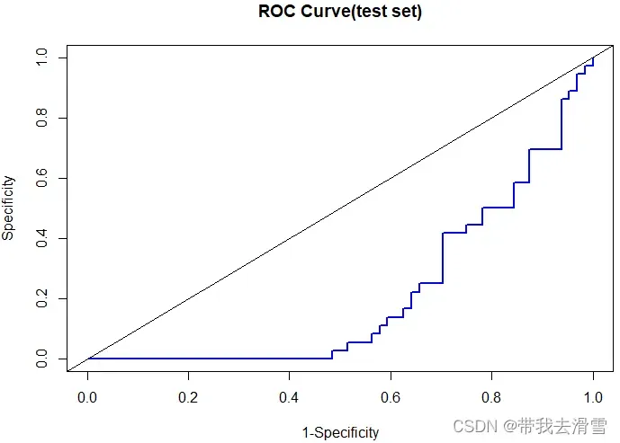
（8）计算 AUC

>aut_test=performance(pred_object,measure=”auc”)
>auc_test@y.values
[1] 0.2122

结果显示，曲线下面积为0.2122。

（9）计算 kappa 值

> install.packages(“vcd”)
> library(vcd)
> Kappa(table)
value ASE z Pr(>|z|)
Unweighted 0.361 0.0973 3.71 0.000205
Weighted 0.361 0.0973 3.71 0.000205

结果显示，在测试集中，kappa值为0.361，表明预测值与实际值之间具有中等一致性。

更多优质内容持续发布中，请移步主页查看。

若有问题可邮箱联系：1736732074@qq.com

博主的WeChat:TCB1736732074

点赞+关注,下次不迷路！

文章出处登录后可见！

已经登录？立即刷新