零基础入门数据挖掘 – 二手车交易价格预测
赛题理解
比赛要求参赛选手根据给定的数据集,建立模型,二手汽车的交易价格。
赛题以预测二手车的交易价格为任务,数据集报名后可见并可下载,该数据来自某交易平台的二手车交易记录,总数据量超过40w,包含31列变量信息,其中15列为匿名变量。为了保证比赛的公平性,将会从中抽取15万条作为训练集,5万条作为测试集A,5万条作为测试集B,同时会对name、model、brand和regionCode等信息进行脱敏。
比赛地址:https://tianchi.aliyun.com/competition/entrance/231784/introduction?spm=5176.12281957.1004.1.38b02448ausjSX
数据形式
训练数据集具有的特征如下:
- name – 汽车编码
- regDate – 汽车注册时间
- model – 车型编码
- brand – 品牌
- bodyType – 车身类型
- fuelType – 燃油类型
- gearbox – 变速箱
- power – 汽车功率
- kilometer – 汽车行驶公里
- notRepairedDamage – 汽车有尚未修复的损坏
- regionCode – 看车地区编码
- seller – 销售方
- offerType – 报价类型
- creatDate – 广告发布时间
- price – 汽车价格(目标列)
- v_0’, ‘v_1’, ‘v_2’, ‘v_3’, ‘v_4’, ‘v_5’, ‘v_6’, ‘v_7’, ‘v_8’, ‘v_9’, ‘v_10’, ‘v_11’, ‘v_12’, ‘v_13’,‘v_14’(根据汽车的评论、标签等大量信息得到的embedding向量)【人工构造 匿名特征】
预测指标
赛题要求采用mae作为评价指标
具体算法
导入相关库
import pandas as pd
import numpy as np
import matplotlib.pyplot as plt
import seaborn as sns
import missingno as msno
import scipy.stats as st
import warnings
warnings.filterwarnings('ignore')
# 解决中文显示问题
plt.rcParams['font.sans-serif'] = ['SimHei']
plt.rcParams['axes.unicode_minus'] = False
数据分析
先读入数据:
train_data = pd.read_csv("used_car_train_20200313.csv", sep = " ")
用excel打开可以看到每一行数据都放下一个单元格中,彼此之间用空格分隔,因此此处需要指定sep为空格,才能够正确读入数据。
观看一下数据:
train_data.head(5).append(train_data.tail(5))
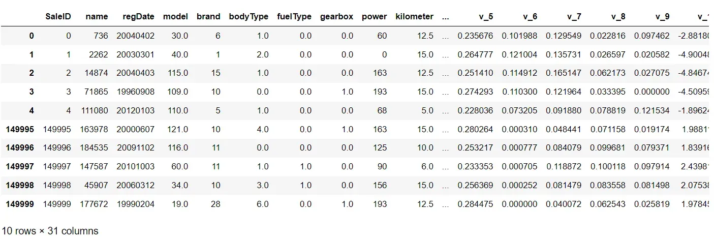
那么下面就开始对数据进行分析。
train_data.columns.values
array(['SaleID', 'name', 'regDate', 'model', 'brand', 'bodyType',
       'fuelType', 'gearbox', 'power', 'kilometer', 'notRepairedDamage',
       'regionCode', 'seller', 'offerType', 'creatDate', 'price', 'v_0',
       'v_1', 'v_2', 'v_3', 'v_4', 'v_5', 'v_6', 'v_7', 'v_8', 'v_9',
       'v_10', 'v_11', 'v_12', 'v_13', 'v_14'], dtype=object)
以上为数据具有的具体特征,那么可以先初步探索一下每个特征的数值类型以及取值等。
train_data.info()
<class 'pandas.core.frame.DataFrame'>
RangeIndex: 150000 entries, 0 to 149999
Data columns (total 31 columns):
 #   Column             Non-Null Count   Dtype
---  ------             --------------   -----
 0   SaleID             150000 non-null  int64
 1   name               150000 non-null  int64
 2   regDate            150000 non-null  int64
 3   model              149999 non-null  float64
 4   brand              150000 non-null  int64
 5   bodyType           145494 non-null  float64
 6   fuelType           141320 non-null  float64
 7   gearbox            144019 non-null  float64
 8   power              150000 non-null  int64
 9   kilometer          150000 non-null  float64
 10  notRepairedDamage  150000 non-null  object
 11  regionCode         150000 non-null  int64
 12  seller             150000 non-null  int64
 13  offerType          150000 non-null  int64
 14  creatDate          150000 non-null  int64
 15  price              150000 non-null  int64
 16  v_0                150000 non-null  float64
 17  v_1                150000 non-null  float64
 18  v_2                150000 non-null  float64
 19  v_3                150000 non-null  float64
 20  v_4                150000 non-null  float64
 21  v_5                150000 non-null  float64
 22  v_6                150000 non-null  float64
 23  v_7                150000 non-null  float64
 24  v_8                150000 non-null  float64
 25  v_9                150000 non-null  float64
 26  v_10               150000 non-null  float64
 27  v_11               150000 non-null  float64
 28  v_12               150000 non-null  float64
 29  v_13               150000 non-null  float64
 30  v_14               150000 non-null  float64
dtypes: float64(20), int64(10), object(1)
memory usage: 35.5+ MB
可以看到除了notRepairedDamage是object类型,其他都是int或者float类型,同时可以看到部分特征还是存在缺失值的,因此这也是后续处理的重要方向。下面查看缺失值的情况:
train_data.isnull().sum()
SaleID                  0
name                    0
regDate                 0
model                   1
brand                   0
bodyType             4506
fuelType             8680
gearbox              5981
power                   0
kilometer               0
notRepairedDamage       0
regionCode              0
seller                  0
offerType               0
creatDate               0
price                   0
v_0                     0
v_1                     0
v_2                     0
v_3                     0
v_4                     0
v_5                     0
v_6                     0
v_7                     0
v_8                     0
v_9                     0
v_10                    0
v_11                    0
v_12                    0
v_13                    0
v_14                    0
dtype: int64
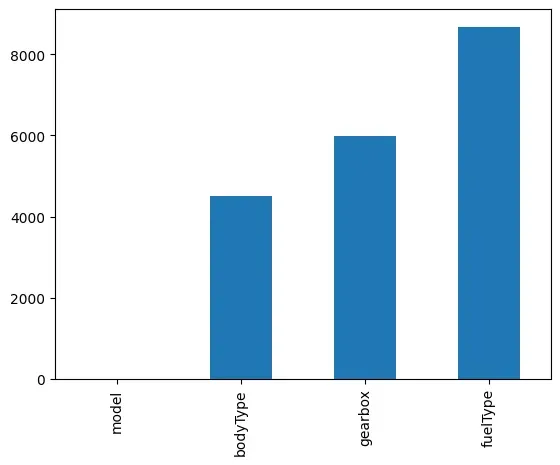
可以看到是部分特征存在较多的缺失值的,因此这是需要处理的部分,下面对缺失值的数目进行可视化展示:
missing = train_data.isnull().sum()
missing = missing[missing > 0]
missing.sort_values(inplace = True)
missing.plot.bar()
我们也可用多种方式来查看缺失值:
msno.matrix(train_data.sample(10000))
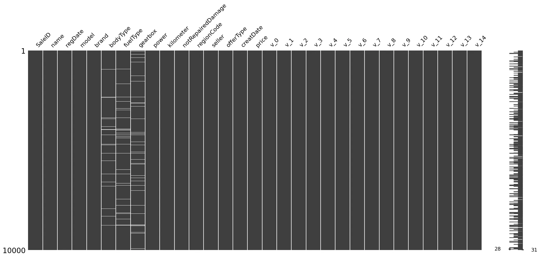
这种图中的白线代表为缺失值,可以看到中间的三个特征存在较多白线,说明其采样10000个的话其中仍然存在较多缺失值。
msno.bar(train_data.sample(10000))
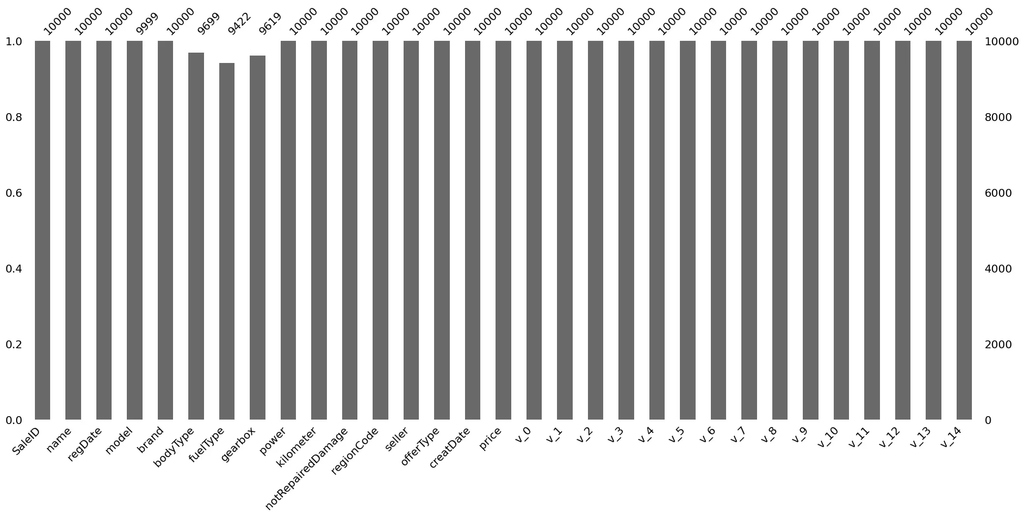
上图中同样是那三个特征,非缺失值的个数也明显比其他特征少。
再回到最开始的数据类型处,我们可以发现notRepairedDamage特征的类型为object,因此我们可以来观察其具有几种取值:
train_data['notRepairedDamage'].value_counts()
0.0    111361
-       24324
1.0     14315
Name: notRepairedDamage, dtype: int64
可以看到其存在”-“取值,这也可以认为是一种缺失值,因此我们可以将”-“转换为nan,然后再统一对nan进行处理。
而为了测试数据集也得到了相同的处理,因此读入数据集并合并:
test_data = pd.read_csv("used_car_testB_20200421.csv", sep = " ")
train_data["origin"] = "train"
test_data["origin"] = "test"
data = pd.concat([train_data, test_data], axis = 0, ignore_index = True)
得到的data数据,是具有20000万条数据。那么可以统一对该数据集的notRepairedDamage特征进行处理:
data['notRepairedDamage'].replace("-", np.nan, inplace = True)
data['notRepairedDamage'].value_counts()
0.0    148585
1.0     19022
Name: notRepairedDamage, dtype: int64
可以看到”-“已经被替换成了nan,因此在计数时没有被考虑在内。
而以下这两种特征的类别严重不平衡,这种情况可以认为它们对于结果的预测并不会起到什么作用:
data['seller'].value_counts()
0    199999
1         1
Name: seller, dtype: int64
data["offerType"].value_counts()
0    200000
Name: offerType, dtype: int64
因此可以对这两个特征进行删除:
del data["seller"]
del data["offerType"]
以上是对特征的初步分析,那么接下来我们对目标列,也就是预测价格进行进一步的分析,先观察其分布情况:
target = train_data['price']
plt.figure(1)
plt.title('Johnson SU')
sns.distplot(target, kde=False, fit=st.johnsonsu)
plt.figure(2)
plt.title('Normal')
sns.distplot(target, kde=False, fit=st.norm)
plt.figure(3)
plt.title('Log Normal')
sns.distplot(target, kde=False, fit=st.lognorm)
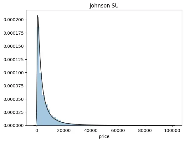
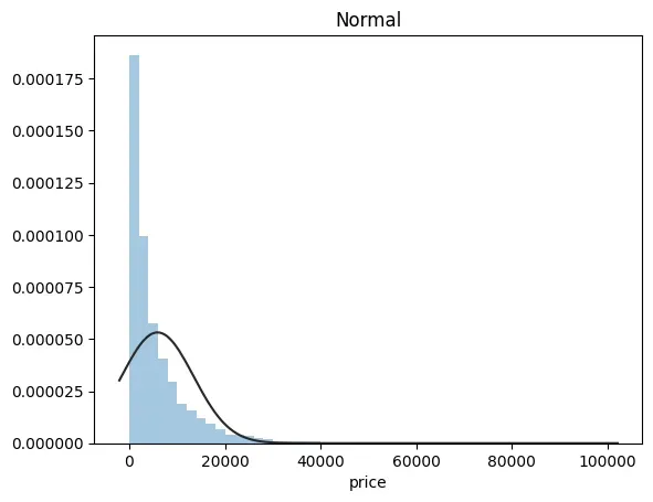
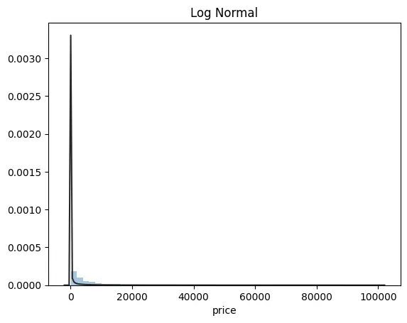
我们可以看到价格的分布是极其不均匀的,这对预测是不利的,部分取值较为极端的例子将会对模型产生较大的影响,并且大部分模型及算法都希望预测的分布能够尽可能地接近正态分布,因此后期需要进行处理,那我们可以从偏度和峰度两个正态分布的角度来观察:
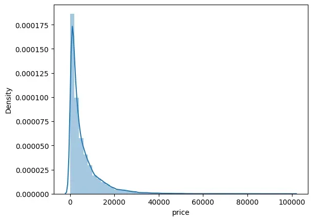
sns.distplot(target);
print("偏度: %f" % target.skew())
print("峰度: %f" % target.kurt())
偏度: 3.346487
峰度: 18.995183
对这种数据分布的处理,通常可以用log来进行压缩转换:
# 需要将其转为正态分布
sns.distplot(np.log(target))
print("偏度: %f" % np.log(target).skew())
print("峰度: %f" % np.log(target).kurt())
偏度: -0.265100
峰度: -0.171801
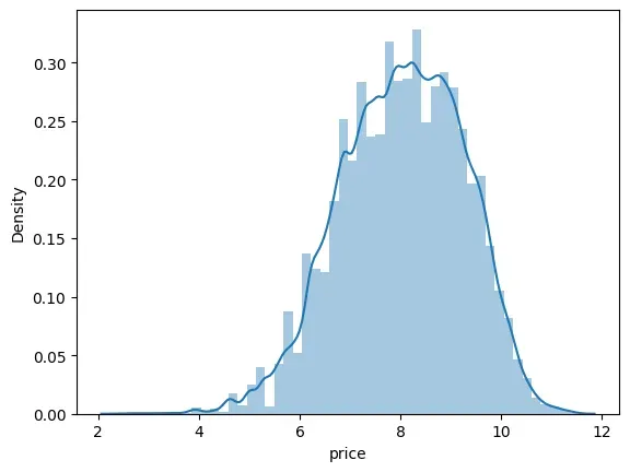
可以看到,经过log变换之后其分布相对好了很多,比较接近正态分布了。
接下来,我们对不同类型的特征进行观察,分别对类别特征和数字特征来观察。由于这里没有在数值类型上加以区分,因此我们需要人工挑选:
numeric_features = ['power', 'kilometer', 'v_0', 'v_1', 'v_2', 'v_3',
                    'v_4', 'v_5', 'v_6', 'v_7', 'v_8', 'v_9', 'v_10',
                    'v_11', 'v_12', 'v_13','v_14' ]

categorical_features = ['name', 'model', 'brand', 'bodyType', 'fuelType','gearbox', 'notRepairedDamage', 'regionCode',]
那么对于类别型特征,我们可以查看其具有多少个取值,是否能够转换one-hot向量:
# 对于类别型的特征需要查看其取值有多少个,能不能转换为onehot
for feature in categorical_features:
    print(feature,"特征有{}个取值".format(train_data[feature].nunique()))
    print(train_data[feature].value_counts())
name 特征有99662个取值
387       282
708       282
55        280
1541      263
203       233
         ...
26403       1
28450       1
32544       1
102174      1
184730      1
Name: name, Length: 99662, dtype: int64
model 特征有248个取值
0.0      11762
19.0      9573
4.0       8445
1.0       6038
29.0      5186
         ...
242.0        2
209.0        2
245.0        2
240.0        2
247.0        1
Name: model, Length: 248, dtype: int64
brand 特征有40个取值
0     31480
4     16737
14    16089
10    14249
1     13794
6     10217
9      7306
5      4665
13     3817
11     2945
3      2461
7      2361
16     2223
8      2077
25     2064
27     2053
21     1547
15     1458
19     1388
20     1236
12     1109
22     1085
26      966
30      940
17      913
24      772
28      649
32      592
29      406
37      333
2       321
31      318
18      316
36      228
34      227
33      218
23      186
35      180
38       65
39        9
Name: brand, dtype: int64
bodyType 特征有8个取值
0.0    41420
1.0    35272
2.0    30324
3.0    13491
4.0     9609
5.0     7607
6.0     6482
7.0     1289
Name: bodyType, dtype: int64
fuelType 特征有7个取值
0.0    91656
1.0    46991
2.0     2212
3.0      262
4.0      118
5.0       45
6.0       36
Name: fuelType, dtype: int64
gearbox 特征有2个取值
0.0    111623
1.0     32396
Name: gearbox, dtype: int64
notRepairedDamage 特征有2个取值
0.0    111361
1.0     14315
Name: notRepairedDamage, dtype: int64
regionCode 特征有7905个取值
419     369
764     258
125     137
176     136
462     134
       ...
7081      1
7243      1
7319      1
7742      1
7960      1
Name: regionCode, Length: 7905, dtype: int64
可以看到name和regionCode 有很多个取值,因此不能转换为onthot,其他是可以的。
而对于数值特征,我们可以来查看其与价格之间的相关性关系,这也有利于我们判断哪些特征更加重要:
numeric_features.append("price")
price_numeric = train_data[numeric_features]
correlation_score = price_numeric.corr() # 得到是一个特征数*特征数的矩阵,元素都行和列对应特征之间的相关性
correlation_score['price'].sort_values(ascending = False)
price        1.000000
v_12         0.692823
v_8          0.685798
v_0          0.628397
power        0.219834
v_5          0.164317
v_2          0.085322
v_6          0.068970
v_1          0.060914
v_14         0.035911
v_13        -0.013993
v_7         -0.053024
v_4         -0.147085
v_9         -0.206205
v_10        -0.246175
v_11        -0.275320
kilometer   -0.440519
v_3         -0.730946
Name: price, dtype: float64
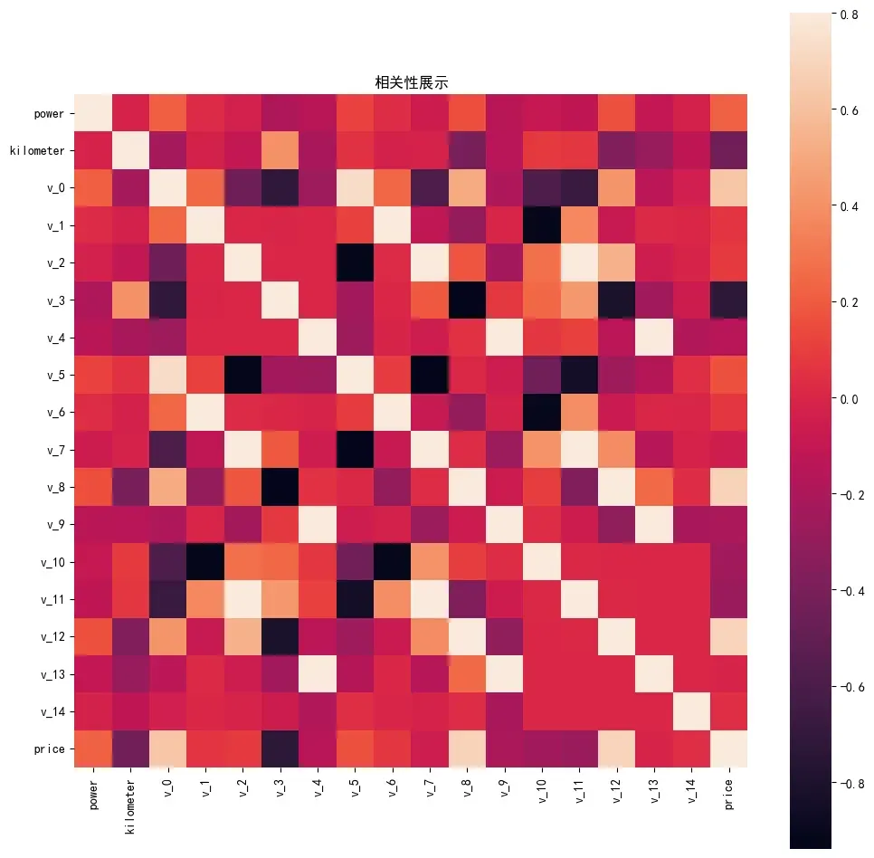
可以看到,例如v14,v13,v1,v7这种跟price之间的相关系数实在是过低,如果是在计算资源有限的情况下可以考虑舍弃这部分特征。我们也可以直观的展示相关性:
fig,ax = plt.subplots(figsize = (12,12))
plt.title("相关性展示")
sns.heatmap(correlation_score, square = True, vmax = 0.8)
对于数值特征来说,我们同样关心其分布,下面先具体分析再说明分布的重要性:
# 查看特征值的偏度和峰度
for col in numeric_features:
    print("{:15}\t Skewness:{:05.2f}\t Kurtosis:{:06.2f}".format(col,
                                                    train_data[col].skew(),
                                                   train_data[col].kurt()))
power          	 Skewness:65.86	 Kurtosis:5733.45
kilometer      	 Skewness:-1.53	 Kurtosis:001.14
v_0            	 Skewness:-1.32	 Kurtosis:003.99
v_1            	 Skewness:00.36	 Kurtosis:-01.75
v_2            	 Skewness:04.84	 Kurtosis:023.86
v_3            	 Skewness:00.11	 Kurtosis:-00.42
v_4            	 Skewness:00.37	 Kurtosis:-00.20
v_5            	 Skewness:-4.74	 Kurtosis:022.93
v_6            	 Skewness:00.37	 Kurtosis:-01.74
v_7            	 Skewness:05.13	 Kurtosis:025.85
v_8            	 Skewness:00.20	 Kurtosis:-00.64
v_9            	 Skewness:00.42	 Kurtosis:-00.32
v_10           	 Skewness:00.03	 Kurtosis:-00.58
v_11           	 Skewness:03.03	 Kurtosis:012.57
v_12           	 Skewness:00.37	 Kurtosis:000.27
v_13           	 Skewness:00.27	 Kurtosis:-00.44
v_14           	 Skewness:-1.19	 Kurtosis:002.39
price          	 Skewness:03.35	 Kurtosis:019.00
可以看到power特征的偏度和峰度都非常大,那么把分布图画出来:
f = pd.melt(train_data, value_vars=numeric_features)
# 这里相当于f是一个两列的矩阵,第一列是原来特征
# 第二列是特征对应的取值,例如power有n个取值,那么它会占据n行,这样叠在一起
g = sns.FacetGrid(f, col="variable",  col_wrap=2, sharex=False, sharey=False)
#g 是产生一个对象,可以用来应用各种图面画图,map应用
# 第一个参数就是dataframe数据,但是要求是长数据,也就是melt处理完的数据
# 第二个参数是用来画图依据的列,valiable是melt处理完,那些特征的列名称
# 而那些值的列名称为value
# 第三个参数col_wrap是代表分成多少列
g = g.map(sns.distplot, "value")
关于melt的使用可以看使用Pandas melt()重塑DataFrame – 知乎 (zhihu.com),我觉得讲得非常容易理解。
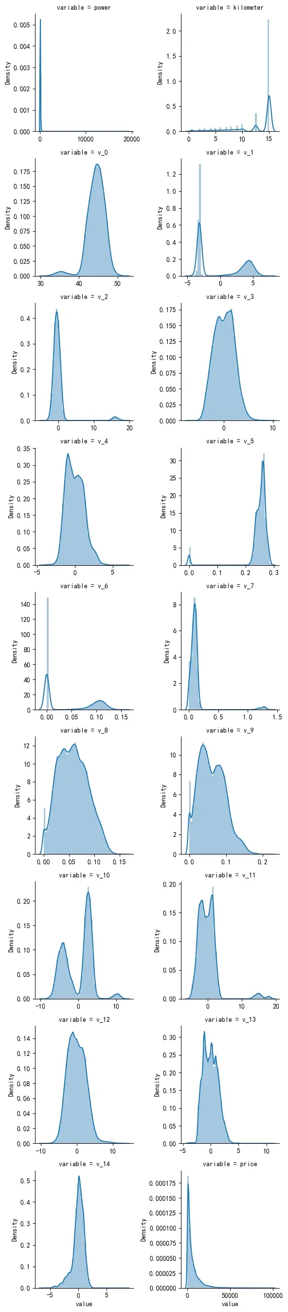
可以看到power的分布非常不均匀,那么跟price同样,如果出现较大极端值的power,就会对结果产生非常严重的影响,这就使得在学习的时候关于power 的权重设定非常不好做。因此后续也需要对这部分进行处理。而匿名的特征的分布相对来说会比较均匀一点,后续可能就不需要进行处理了。
还可以通过散点图来观察两两之间大概的关系分布:
sns.pairplot(train_data[numeric_features], size = 2, kind = "scatter",diag_kind = "kde")

(这部分就自己看自己发挥吧)
下面继续回到类别型特征,由于其中存在nan不方便我们画图展示,因此我们可以先将nan进行替换,方便画图展示:
# 下面对类别特征做处理
categorical_features_2 = ['model',
 'brand',
 'bodyType',
 'fuelType',
 'gearbox',
 'notRepairedDamage']
for c in categorical_features_2:
    train_data[c] = train_data[c].astype("category")
    # 将这些的类型转换为分类类型,不保留原来的int或者float类型
    if train_data[c].isnull().any():
        # 如果该列存在nan的话
        train_data[c] = train_data[c].cat.add_categories(['Missing'])
        # 增加一个新的分类为missing,用它来填充那些nan,代表缺失值,
        # 这样在后面画图方便展示
        train_data[c] = train_data[c].fillna('Missing')
下面通过箱型图来对类别特征的每个取值进行直观展示:
def bar_plot(x, y, **kwargs):
    sns.barplot(x = x, y = y)
    x = plt.xticks(rotation = 90)

f = pd.melt(train_data, id_vars = ['price'], value_vars = categorical_features_2)
g = sns.FacetGrid(f, col = 'variable', col_wrap = 2, sharex = False, sharey = False)
g = g.map(bar_plot, "value", "price")
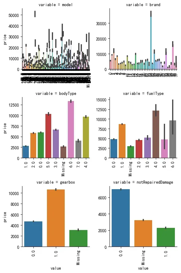
这可以看到类别型特征相对来说分布也不会出现极端情况。
特征工程
在特征处理中,最重要的我觉得是对异常数据的处理。之前我们已经看到了power特征的分布尤为不均匀,那么这部分有两种处理方式,一种是对极端值进行舍去,一部分是采用log的方式进行压缩,那么这里都进行介绍。
首先是对极端值进行舍去,那么可以采用箱型图来协助判断,下面封装一个函数实现:
# 主要就是power的值分布太过于异常,那么可以对一些进行处理,删除掉
# 下面定义一个函数用来处理异常值
def outliers_proc(data, col_name, scale = 3):
    # data:原数据
    # col_name:要处理异常值的列名称
    # scale:用来控制删除尺度的
    def box_plot_outliers(data_ser, box_scale):
        iqr = box_scale * (data_ser.quantile(0.75) - data_ser.quantile(0.25))
        # quantile是取出数据对应分位数的数值
        val_low = data_ser.quantile(0.25) - iqr # 下界
        val_up = data_ser.quantile(0.75) + iqr # 上界
        rule_low = (data_ser < val_low) # 筛选出小于下界的索引
        rule_up = (data_ser > val_up) # 筛选出大于上界的索引
        return (rule_low, rule_up),(val_low, val_up)

    data_n = data.copy()
    data_series = data_n[col_name]  # 取出对应数据
    rule, values = box_plot_outliers(data_series, box_scale = scale)
    index = np.arange(data_series.shape[0])[rule[0] | rule[1]]
    # 先产生0到n-1,然后再用索引把其中处于异常值的索引取出来
    print("Delete number is {}".format(len(index)))
    data_n = data_n.drop(index) # 整行数据都丢弃
    data_n.reset_index(drop = True, inplace = True)  # 重新设置索引
    print("Now column number is:{}".format(data_n.shape[0]))
    index_low = np.arange(data_series.shape[0])[rule[0]]
    outliers = data_series.iloc[index_low]  # 小于下界的值
    print("Description of data less than the lower bound is:")
    print(pd.Series(outliers).describe())
    index_up = np.arange(data_series.shape[0])[rule[1]]
    outliers = data_series.iloc[index_up]
    print("Description of data larger than the lower bound is:")
    print(pd.Series(outliers).describe())
    fig, axes = plt.subplots(1,2,figsize = (10,7))
    ax1 = sns.boxplot(y = data[col_name], data = data, palette = "Set1", ax = axes[0])
    ax1.set_title("处理异常值前")
    ax2 = sns.boxplot(y = data_n[col_name], data = data_n, palette = "Set1", ax = axes[1])
    ax2.set_title("处理异常值后")
    return data_n
我们应用于power数据集尝试:
train_data_delete_after = outliers_proc(train_data, "power", scale =3)
Delete number is 963
Now column number is:149037
Description of data less than the lower bound is:
count    0.0
mean     NaN
std      NaN
min      NaN
25%      NaN
50%      NaN
75%      NaN
max      NaN
Name: power, dtype: float64
Description of data larger than the lower bound is:
count      963.000000
mean       846.836968
std       1929.418081
min        376.000000
25%        400.000000
50%        436.000000
75%        514.000000
max      19312.000000
Name: power, dtype: float64
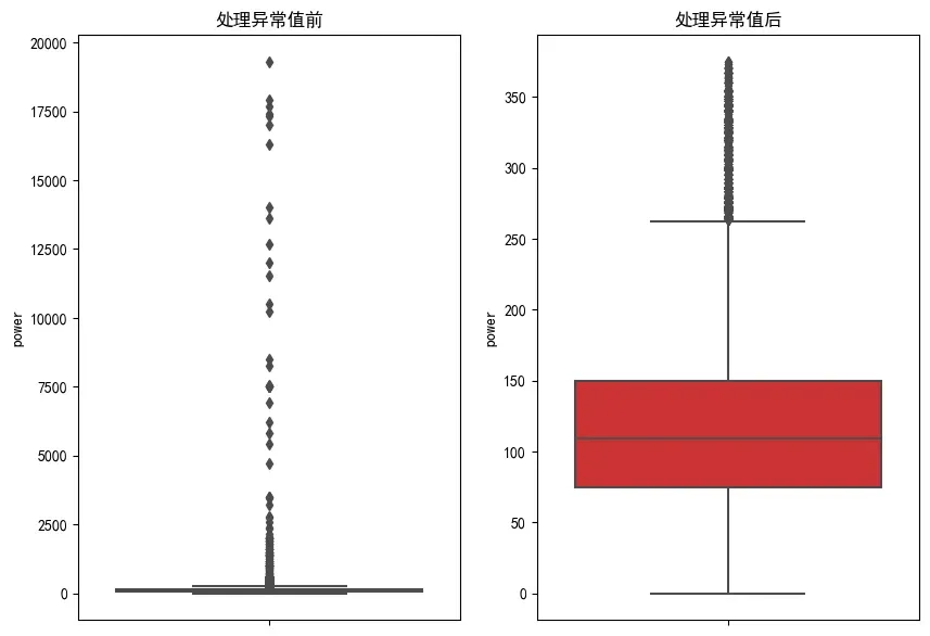
可以看到总共删除了900多条数据,使得最终的箱型图也正常许多。
那么另外一种方法就是采用log进行压缩,但这里因为我还想用power进行数据分桶,构造出一个power等级的特征,因此我就先构造再进行压缩:
bin_power = [i*10 for i in range(31)]
data["power_bin"] = pd.cut(data["power"],bin_power,right = False,labels = False)
这种方法就是将power按照bin_power的数值进行分段,最低一段在新特征中取值为1,以此类推,但是这样会导致大于最大一段的取值为nan,也就是power取值大于300的在power_bin中取值为nan,因此可以设置其等级为31来处理:
data['power_bin'] = data['power_bin'].fillna(31)
那么对于power现在就可以用log进行压缩了:
data['power'] = np.log(data['power'] + 1)
接下来进行新特征的构造。
首先是使用时间,我们可以用creatDate减去regDate来表示:
data["use_time"] = (pd.to_datetime(data['creatDate'],format = "%Y%m%d",errors = "coerce")
                        - pd.to_datetime(data["regDate"], format = "%Y%m%d", errors = "coerce")).dt.days
# errors是当格式转换错误就赋予nan
而这种处理方法由于部分数据日期的缺失,会导致存在缺失值,那么我的处理方法是填充为均值,但是测试集的填充也需要用训练数据集的均值来填充,因此我放到后面划分的时候再来处理。
下面是对品牌的销售统计量创造特征,因为要计算某个品牌的销售均值、最大值、方差等等数据,因此我们需要在训练数据集上计算,测试数据集是未知的,计算完毕后再根据品牌一一对应填上数值即可:
# 计算某个品牌的各种统计数目量
train_gb = train_data.groupby("brand")
all_info = {}
for kind, kind_data in train_gb:
    info = {}
    kind_data = kind_data[kind_data["price"] > 0]
    # 把价格小于0的可能存在的异常值去除
    info["brand_amount"] = len(kind_data) # 该品牌的数量
    info["brand_price_max"] = kind_data.price.max() # 该品牌价格最大值
    info["brand_price_min"] = kind_data.price.min() # 该品牌价格最小值
    info["brand_price_median"] = kind_data.price.median() # 该品牌价格中位数
    info["brand_price_sum"] = kind_data.price.sum() # 该品牌价格总和
    info["brand_price_std"] = kind_data.price.std() # 方差
    info["brand_price_average"] = round(kind_data.price.sum() / (len(kind_data) + 1), 2)
    # 均值,保留两位小数
    all_info[kind] = info
brand_feature = pd.DataFrame(all_info).T.reset_index().rename(columns = {"index":"brand"})
这里的brand_feature获得方法可能有点复杂,我一步步解释出来:
brand_feature = pd.DataFrame(all_info)
brand_feature
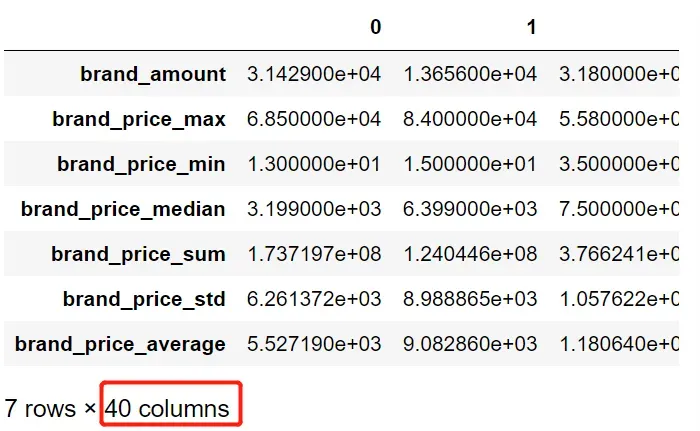
这里是7个统计量特征作为索引,然后有40列代表有40个品牌。
brand_feature = pd.DataFrame(all_info).T.reset_index()
brand_feature
转置后重新设置索引,也就是:
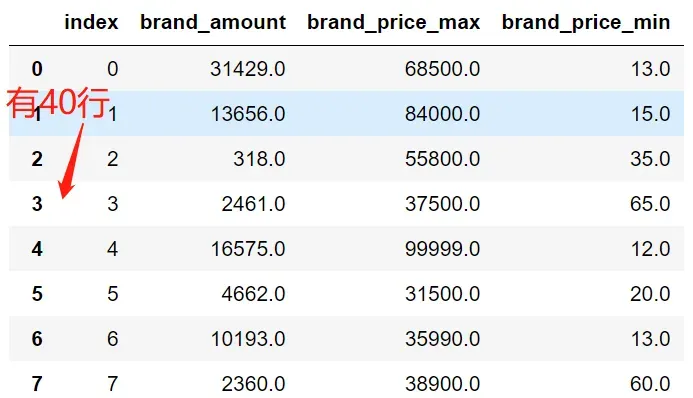
将品牌统计量作为列,然后加入一个列为index,可以认为是品牌的取值。
brand_feature = pd.DataFrame(all_info).T.reset_index().rename(columns = {"index":"brand"})
brand_feature
这一个就是将index更名为brand,这一列就是品牌的取值,方便我们后续融合到data中:
data = data.merge(brand_feature, how='left', on='brand')
这就是将data中的brand取值和刚才那个矩阵中的取值一一对应,然后取出对应的特征各个值,作为新的特征。
接下来需要对大部分数据进行归一化:
def max_min(x):
    return (x - np.min(x)) / (np.max(x) - np.min(x))
for feature in ["brand_amount","brand_price_average","brand_price_max",
                "brand_price_median","brand_price_min","brand_price_std",
               "brand_price_sum","power","kilometer"]:
    data[feature] = max_min(data[feature])
对类别特征进行encoder:
# 对类别特征转换为onehot
data = pd.get_dummies(data, columns=['model', 'brand', 'bodyType','fuelType','gearbox',
                                     'notRepairedDamage', 'power_bin'],dummy_na=True)
对没用的特征可以进行删除了:
data = data.drop(['creatDate',"regDate", "regionCode"], axis = 1)
至此,关于特征的处理工作基本上就完成了,但是这只是简单的处理方式,可以去探索更加深度的特征信息(我不会哈哈哈哈)。
建立模型
先处理数据集:
use_feature = [x for x in data.columns if x not in ['SaleID',"name","price","origin"]]
target = data[data["origin"] == "train"]["price"]
target_lg = (np.log(target+1))

train_x = data[data["origin"] == "train"][use_feature]
test_x = data[data["origin"] == "test"][use_feature]

train_x["use_time"] = train_x["use_time"].fillna(train_x["use_time"].mean())

test_x["use_time"] = test_x["use_time"].fillna(train_x["use_time"].mean())# 用训练数据集的均值填充

train_x.shape
(150000, 371)
可以看看训练数据是否还存在缺失值:
test_x.isnull().sum()
power                    0
kilometer                0
v_0                      0
v_1                      0
v_2                      0
v_3                      0
v_4                      0
v_5                      0
v_6                      0
v_7                      0
v_8                      0
v_9                      0
v_10                     0
v_11                     0
v_12                     0
v_13                     0
v_14                     0
use_time                 0
brand_amount             0
brand_price_max          0
brand_price_min          0
brand_price_median       0
brand_price_sum          0
brand_price_std          0
brand_price_average      0
model_0.0                0
model_1.0                0
model_2.0                0
model_3.0                0
model_4.0                0
model_5.0                0
model_6.0                0
model_7.0                0
model_8.0                0
model_9.0                0
model_10.0               0
model_11.0               0
model_12.0               0
model_13.0               0
model_14.0               0
model_15.0               0
model_16.0               0
model_17.0               0
model_18.0               0
model_19.0               0
model_20.0               0
model_21.0               0
model_22.0               0
model_23.0               0
model_24.0               0
model_25.0               0
model_26.0               0
model_27.0               0
model_28.0               0
model_29.0               0
model_30.0               0
model_31.0               0
model_32.0               0
model_33.0               0
model_34.0               0
model_35.0               0
model_36.0               0
model_37.0               0
model_38.0               0
model_39.0               0
model_40.0               0
model_41.0               0
model_42.0               0
model_43.0               0
model_44.0               0
model_45.0               0
model_46.0               0
model_47.0               0
model_48.0               0
model_49.0               0
model_50.0               0
model_51.0               0
model_52.0               0
model_53.0               0
model_54.0               0
model_55.0               0
model_56.0               0
model_57.0               0
model_58.0               0
model_59.0               0
model_60.0               0
model_61.0               0
model_62.0               0
model_63.0               0
model_64.0               0
model_65.0               0
model_66.0               0
model_67.0               0
model_68.0               0
model_69.0               0
model_70.0               0
model_71.0               0
model_72.0               0
model_73.0               0
model_74.0               0
model_75.0               0
model_76.0               0
model_77.0               0
model_78.0               0
model_79.0               0
model_80.0               0
model_81.0               0
model_82.0               0
model_83.0               0
model_84.0               0
model_85.0               0
model_86.0               0
model_87.0               0
model_88.0               0
model_89.0               0
model_90.0               0
model_91.0               0
model_92.0               0
model_93.0               0
model_94.0               0
model_95.0               0
model_96.0               0
model_97.0               0
model_98.0               0
model_99.0               0
model_100.0              0
model_101.0              0
model_102.0              0
model_103.0              0
model_104.0              0
model_105.0              0
model_106.0              0
model_107.0              0
model_108.0              0
model_109.0              0
model_110.0              0
model_111.0              0
model_112.0              0
model_113.0              0
model_114.0              0
model_115.0              0
model_116.0              0
model_117.0              0
model_118.0              0
model_119.0              0
model_120.0              0
model_121.0              0
model_122.0              0
model_123.0              0
model_124.0              0
model_125.0              0
model_126.0              0
model_127.0              0
model_128.0              0
model_129.0              0
model_130.0              0
model_131.0              0
model_132.0              0
model_133.0              0
model_134.0              0
model_135.0              0
model_136.0              0
model_137.0              0
model_138.0              0
model_139.0              0
model_140.0              0
model_141.0              0
model_142.0              0
model_143.0              0
model_144.0              0
model_145.0              0
model_146.0              0
model_147.0              0
model_148.0              0
model_149.0              0
model_150.0              0
model_151.0              0
model_152.0              0
model_153.0              0
model_154.0              0
model_155.0              0
model_156.0              0
model_157.0              0
model_158.0              0
model_159.0              0
model_160.0              0
model_161.0              0
model_162.0              0
model_163.0              0
model_164.0              0
model_165.0              0
model_166.0              0
model_167.0              0
model_168.0              0
model_169.0              0
model_170.0              0
model_171.0              0
model_172.0              0
model_173.0              0
model_174.0              0
model_175.0              0
model_176.0              0
model_177.0              0
model_178.0              0
model_179.0              0
model_180.0              0
model_181.0              0
model_182.0              0
model_183.0              0
model_184.0              0
model_185.0              0
model_186.0              0
model_187.0              0
model_188.0              0
model_189.0              0
model_190.0              0
model_191.0              0
model_192.0              0
model_193.0              0
model_194.0              0
model_195.0              0
model_196.0              0
model_197.0              0
model_198.0              0
model_199.0              0
model_200.0              0
model_201.0              0
model_202.0              0
model_203.0              0
model_204.0              0
model_205.0              0
model_206.0              0
model_207.0              0
model_208.0              0
model_209.0              0
model_210.0              0
model_211.0              0
model_212.0              0
model_213.0              0
model_214.0              0
model_215.0              0
model_216.0              0
model_217.0              0
model_218.0              0
model_219.0              0
model_220.0              0
model_221.0              0
model_222.0              0
model_223.0              0
model_224.0              0
model_225.0              0
model_226.0              0
model_227.0              0
model_228.0              0
model_229.0              0
model_230.0              0
model_231.0              0
model_232.0              0
model_233.0              0
model_234.0              0
model_235.0              0
model_236.0              0
model_237.0              0
model_238.0              0
model_239.0              0
model_240.0              0
model_241.0              0
model_242.0              0
model_243.0              0
model_244.0              0
model_245.0              0
model_246.0              0
model_247.0              0
model_nan                0
brand_0.0                0
brand_1.0                0
brand_2.0                0
brand_3.0                0
brand_4.0                0
brand_5.0                0
brand_6.0                0
brand_7.0                0
brand_8.0                0
brand_9.0                0
brand_10.0               0
brand_11.0               0
brand_12.0               0
brand_13.0               0
brand_14.0               0
brand_15.0               0
brand_16.0               0
brand_17.0               0
brand_18.0               0
brand_19.0               0
brand_20.0               0
brand_21.0               0
brand_22.0               0
brand_23.0               0
brand_24.0               0
brand_25.0               0
brand_26.0               0
brand_27.0               0
brand_28.0               0
brand_29.0               0
brand_30.0               0
brand_31.0               0
brand_32.0               0
brand_33.0               0
brand_34.0               0
brand_35.0               0
brand_36.0               0
brand_37.0               0
brand_38.0               0
brand_39.0               0
brand_nan                0
bodyType_0.0             0
bodyType_1.0             0
bodyType_2.0             0
bodyType_3.0             0
bodyType_4.0             0
bodyType_5.0             0
bodyType_6.0             0
bodyType_7.0             0
bodyType_nan             0
fuelType_0.0             0
fuelType_1.0             0
fuelType_2.0             0
fuelType_3.0             0
fuelType_4.0             0
fuelType_5.0             0
fuelType_6.0             0
fuelType_nan             0
gearbox_0.0              0
gearbox_1.0              0
gearbox_nan              0
notRepairedDamage_0.0    0
notRepairedDamage_1.0    0
notRepairedDamage_nan    0
power_bin_0.0            0
power_bin_1.0            0
power_bin_2.0            0
power_bin_3.0            0
power_bin_4.0            0
power_bin_5.0            0
power_bin_6.0            0
power_bin_7.0            0
power_bin_8.0            0
power_bin_9.0            0
power_bin_10.0           0
power_bin_11.0           0
power_bin_12.0           0
power_bin_13.0           0
power_bin_14.0           0
power_bin_15.0           0
power_bin_16.0           0
power_bin_17.0           0
power_bin_18.0           0
power_bin_19.0           0
power_bin_20.0           0
power_bin_21.0           0
power_bin_22.0           0
power_bin_23.0           0
power_bin_24.0           0
power_bin_25.0           0
power_bin_26.0           0
power_bin_27.0           0
power_bin_28.0           0
power_bin_29.0           0
power_bin_31.0           0
power_bin_nan            0
dtype: int64
可以看到都没有缺失值了,因此接下来可以用来选择模型了。
由于现实原因(电脑跑不动xgboost)因此我选择了lightGBM和随机森林、梯度提升决策树三种,然后再用模型融合,具体代码如下:
from sklearn import metrics
import matplotlib.pyplot as plt
from sklearn.metrics import roc_auc_score, roc_curve, mean_squared_error,mean_absolute_error, f1_score
import lightgbm as lgb
import xgboost as xgb
from sklearn.ensemble import RandomForestRegressor as rfr
from sklearn.model_selection import  KFold, StratifiedKFold,GroupKFold, RepeatedKFold
from sklearn.model_selection import train_test_split
from sklearn.model_selection import GridSearchCV
from sklearn import preprocessing
from sklearn.metrics import mean_absolute_error
from sklearn.ensemble import GradientBoostingRegressor as gbr
from sklearn.linear_model import LinearRegression as lr
lightGBM:
lgb_param = {  # 这是训练的参数列表
    "num_leaves":7,
    "min_data_in_leaf": 20,  # 一个叶子上最小分配到的数量,用来处理过拟合
    "objective": "regression",  # 设置类型为回归
    "max_depth": -1,  # 限制树的最大深度,-1代表没有限制
    "learning_rate": 0.003,
    "boosting": "gbdt",  # 用gbdt算法
    "feature_fraction": 0.50,  # 每次迭代时使用18%的特征参与建树,引入特征子空间的多样性
    "bagging_freq": 1,  # 每一次迭代都执行bagging
    "bagging_fraction": 0.55,  # 每次bagging在不进行重采样的情况下随机选择55%数据训练
    "bagging_seed": 1,
    "metric": 'mean_absolute_error',
    "lambda_l1": 0.5,
    "lambda_l2": 0.5,
    "verbosity": -1  # 打印消息的详细程度
}
folds = StratifiedKFold(n_splits=5, shuffle=True, random_state = 4)
# 产生一个容器,可以用来对对数据集进行打乱的5次切分,以此来进行五折交叉验证
valid_lgb = np.zeros(len(train_x))
predictions_lgb = np.zeros(len(test_x))


for fold_, (train_idx, valid_idx) in enumerate(folds.split(train_x, target)):
    # 切分后返回的训练集和验证集的索引
    print("fold n{}".format(fold_+1))  # 当前第几折
    train_data_now = lgb.Dataset(train_x.iloc[train_idx], target_lg[train_idx])
    valid_data_now = lgb.Dataset(train_x.iloc[valid_idx], target_lg[valid_idx])
    # 取出数据并转换为lgb的数据
    num_round = 10000
    lgb_model = lgb.train(lgb_param, train_data_now, num_round,
                        valid_sets=[train_data_now, valid_data_now], verbose_eval=500,
                       early_stopping_rounds = 800)
    valid_lgb[valid_idx] = lgb_model.predict(train_x.iloc[valid_idx],
                                             num_iteration=lgb_model.best_iteration)
    predictions_lgb += lgb_model.predict(test_x, num_iteration=
                                           lgb_model.best_iteration) / folds.n_splits
    # 这是将预测概率进行平均
print("CV score: {:<8.8f}".format(mean_absolute_error(valid_lgb, target_lg)))
这里需要注意我进入训练时split用的是target,而在其中价格用的是target_lg,因为target是原始的价格,可以认为是离散的取值,但是我target_lg经过np.log之后,我再用target_lg进行split时就会报错,为:
Supported target types are: (‘binary’, ‘multiclass’). Got ‘continuous’ instead.
我认为是np.nan将其转换为了连续型数值,而不是原来的离散型数值取值,因此我只能用target去产生切片索引。
CV score: 0.15345674
同样,观察一下特征重要性:
pd.set_option("display.max_columns", None)  # 设置可以显示的最大行和最大列
pd.set_option('display.max_rows', None)  # 如果超过就显示省略号,none表示不省略
#设置value的显示长度为100,默认为50
pd.set_option('max_colwidth',100)
# 创建,然后只有一列就是刚才所使用的的特征
df = pd.DataFrame(train_x.columns.tolist(), columns=['feature'])
df['importance'] = list(lgb_model.feature_importance())
df = df.sort_values(by='importance', ascending=False)  # 降序排列
plt.figure(figsize = (14,28))
sns.barplot(x='importance', y='feature', data = df.head(50))# 取出前五十个画图
plt.title('Features importance (averaged/folds)')
plt.tight_layout()  # 自动调整适应范围
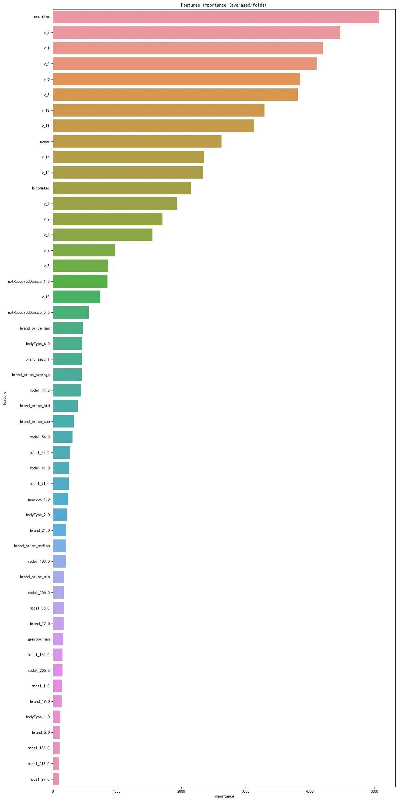
可以看到使用时间遥遥领先。
随机森林:
#RandomForestRegressor随机森林
folds = KFold(n_splits=5, shuffle=True, random_state=2019)
valid_rfr = np.zeros(len(train_x))
predictions_rfr = np.zeros(len(test_x))

for fold_, (trn_idx, val_idx) in enumerate(folds.split(train_x, target)):
    print("fold n°{}".format(fold_+1))
    tr_x = train_x.iloc[trn_idx]
    tr_y = target_lg[trn_idx]
    rfr_model = rfr(n_estimators=1600,max_depth=9, min_samples_leaf=9,
                  min_weight_fraction_leaf=0.0,max_features=0.25,
                  verbose=1,n_jobs=-1) #并行化
    #verbose = 0 为不在标准输出流输出日志信息
#verbose = 1 为输出进度条记录
#verbose = 2 为每个epoch输出一行记录
    rfr_model.fit(tr_x,tr_y)
    valid_rfr[val_idx] = rfr_model.predict(train_x.iloc[val_idx])

    predictions_rfr += rfr_model.predict(test_x) / folds.n_splits

print("CV score: {:<8.8f}".format(mean_absolute_error(valid_rfr, target_lg)))
CV score: 0.17160127
梯度提升:
#GradientBoostingRegressor梯度提升决策树
folds = StratifiedKFold(n_splits=5, shuffle=True, random_state=2018)
valid_gbr = np.zeros(len(train_x))
predictions_gbr = np.zeros(len(test_x))

for fold_, (trn_idx, val_idx) in enumerate(folds.split(train_x, target)):
    print("fold n°{}".format(fold_+1))
    tr_x = train_x.iloc[trn_idx]
    tr_y = target_lg[trn_idx]
    gbr_model = gbr(n_estimators=100, learning_rate=0.1,subsample=0.65 ,max_depth=7,
                    min_samples_leaf=20, max_features=0.22,verbose=1)
    gbr_model.fit(tr_x,tr_y)
    valid_gbr[val_idx] = gbr_model.predict(train_x.iloc[val_idx])

    predictions_gbr += gbr_model.predict(test_x) / folds.n_splits

print("CV score: {:<8.8f}".format(mean_absolute_error(valid_gbr, target_lg)))
CV score: 0.14386158
下面用逻辑回归对这三种模型进行融合:
train_stack2 = np.vstack([valid_lgb, valid_rfr, valid_gbr]).transpose()
test_stack2 = np.vstack([predictions_lgb, predictions_rfr,predictions_gbr]).transpose()
#交叉验证:5折,重复2次
folds_stack = RepeatedKFold(n_splits=5, n_repeats=2, random_state=7)
valid_stack2 = np.zeros(train_stack2.shape[0])
predictions_lr2 = np.zeros(test_stack2.shape[0])

for fold_, (trn_idx, val_idx) in enumerate(folds_stack.split(train_stack2,target)):
    print("fold {}".format(fold_))
    trn_data, trn_y = train_stack2[trn_idx], target_lg.iloc[trn_idx].values
    val_data, val_y = train_stack2[val_idx], target_lg.iloc[val_idx].values
    #Kernel Ridge Regression
    lr2 = lr()
    lr2.fit(trn_data, trn_y)

    valid_stack2[val_idx] = lr2.predict(val_data)
    predictions_lr2 += lr2.predict(test_stack2) / 10

print("CV score: {:<8.8f}".format(mean_absolute_error(target_lg.values, valid_stack2)))
CV score: 0.14343221
那么就可以将预测结果先经过exp得到真正结果就去提交啦!
prediction_test = np.exp(predictions_lr2) - 1
test_submission = pd.read_csv("used_car_testB_20200421.csv", sep = " ")
test_submission["price"] = prediction_test
feature_submission = ["SaleID","price"]
sub = test_submission[feature_submission]
sub.to_csv("mysubmission.csv",index = False)
上述是直接指定参数,那么接下来我会对lightGBM进行调参,看看是否能够取得更好的结果:
# 下面对lightgbm调参
# 构建数据集
train_y = target_lg
x_train, x_valid, y_train, y_valid = train_test_split(train_x, train_y,
                                                      random_state = 1, test_size = 0.2)
# 数据转换
lgb_train = lgb.Dataset(x_train, y_train, free_raw_data = False)
lgb_valid = lgb.Dataset(x_valid, y_valid, reference=lgb_train,free_raw_data=False)

# 设置初始参数
params = {
    "boosting_type":"gbdt",
    "objective":"regression",
    "metric":"mae",
    "nthread":4,
    "learning_rate":0.1,
    "verbosity": -1
}

# 交叉验证调参
print("交叉验证")
min_mae = 10000
best_params = {}

print("调参1:提高准确率")
for num_leaves in range(5,100,5):
    for max_depth in range(3,10,1):
        params["num_leaves"] = num_leaves
        params["max_depth"] = max_depth
        cv_results = lgb.cv(params, lgb_train,seed = 1,nfold =5,
                           metrics=["mae"], early_stopping_rounds = 15,stratified=False,
                           verbose_eval = True)
        mean_mae = pd.Series(cv_results['l1-mean']).max()
        boost_rounds = pd.Series(cv_results["l1-mean"]).idxmax()
        if mean_mae <= min_mae:
            min_mae = mean_mae
            best_params["num_leaves"] = num_leaves
            best_params["max_depth"] = max_depth
if "num_leaves" and "max_depth" in best_params.keys():
    params["num_leaves"] = best_params["num_leaves"]
    params["max_depth"] = best_params["max_depth"]

print("调参2:降低过拟合")
for max_bin in range(5,256,10):
    for min_data_in_leaf in range(1,102,10):
            params['max_bin'] = max_bin
            params['min_data_in_leaf'] = min_data_in_leaf

            cv_results = lgb.cv(
                                params,
                                lgb_train,
                                seed=1,
                                nfold=5,
                                metrics=['mae'],
                                early_stopping_rounds=10,
                                verbose_eval=True,
                                stratified=False
                                )

            mean_mae = pd.Series(cv_results['l1-mean']).max()
            boost_rounds = pd.Series(cv_results['l1-mean']).idxmax()

            if mean_mae <= min_mae:
                min_mae = mean_mae
                best_params['max_bin']= max_bin
                best_params['min_data_in_leaf'] = min_data_in_leaf
if 'max_bin' and 'min_data_in_leaf' in best_params.keys():
    params['min_data_in_leaf'] = best_params['min_data_in_leaf']
    params['max_bin'] = best_params['max_bin']

print("调参3:降低过拟合")
for feature_fraction in [0.6,0.7,0.8,0.9,1.0]:
    for bagging_fraction in [0.6,0.7,0.8,0.9,1.0]:
        for bagging_freq in range(0,50,5):
            params['feature_fraction'] = feature_fraction
            params['bagging_fraction'] = bagging_fraction
            params['bagging_freq'] = bagging_freq

            cv_results = lgb.cv(
                                params,
                                lgb_train,
                                seed=1,
                                nfold=5,
                                metrics=['mae'],
                                early_stopping_rounds=10,
                                verbose_eval=True,
                                stratified=False
                                )

            mean_mae = pd.Series(cv_results['l1-mean']).max()
            boost_rounds = pd.Series(cv_results['l1-mean']).idxmax()

            if mean_mae <= min_mae:
                min_mae = mean_mae
                best_params['feature_fraction'] = feature_fraction
                best_params['bagging_fraction'] = bagging_fraction
                best_params['bagging_freq'] = bagging_freq

if 'feature_fraction' and 'bagging_fraction' and 'bagging_freq' in best_params.keys():
    params['feature_fraction'] = best_params['feature_fraction']
    params['bagging_fraction'] = best_params['bagging_fraction']
    params['bagging_freq'] = best_params['bagging_freq']

print("调参4:降低过拟合")
for lambda_l1 in [1e-5,1e-3,1e-1,0.0,0.1,0.3,0.5,0.7,0.9,1.0]:
    for lambda_l2 in [1e-5,1e-3,1e-1,0.0,0.1,0.4,0.6,0.7,0.9,1.0]:
        params['lambda_l1'] = lambda_l1
        params['lambda_l2'] = lambda_l2
        cv_results = lgb.cv(
                            params,
                            lgb_train,
                            seed=1,
                            nfold=5,
                            metrics=['mae'],
                            early_stopping_rounds=10,
                            verbose_eval=True,
                            stratified=False
                            )

        mean_mae = pd.Series(cv_results['l1-mean']).max()
        boost_rounds = pd.Series(cv_results['l1-mean']).idxmax()

        if mean_mae <= min_mae:
            min_mae = mean_mae
            best_params['lambda_l1'] = lambda_l1
            best_params['lambda_l2'] = lambda_l2
if 'lambda_l1' and 'lambda_l2' in best_params.keys():
    params['lambda_l1'] = best_params['lambda_l1']
    params['lambda_l2'] = best_params['lambda_l2']


print("调参5:降低过拟合2")
for min_split_gain in [0.0,0.1,0.2,0.3,0.4,0.5,0.6,0.7,0.8,0.9,1.0]:
    params['min_split_gain'] = min_split_gain

    cv_results = lgb.cv(
                        params,
                        lgb_train,
                        seed=1,
                        nfold=5,
                        metrics=['mae'],
                        early_stopping_rounds=10,
                        verbose_eval=True,
                        stratified=False
                        )

    mean_mae = pd.Series(cv_results['l1-mean']).max()
    boost_rounds = pd.Series(cv_results['l1-mean']).idxmax()

    if mean_mae <= min_mae:
        min_mae = mean_mae
        best_params['min_split_gain'] = min_split_gain

if 'min_split_gain' in best_params.keys():
    params['min_split_gain'] = best_params['min_split_gain']

print(best_params)
注意在lgb.cv中要设置参数stratified=False,同样是之间那个连续与离散的问题!
{'num_leaves': 95, 'max_depth': 9, 'max_bin': 215, 'min_data_in_leaf': 71, 'feature_fraction': 1.0, 'bagging_fraction': 1.0, 'bagging_freq': 45, 'lambda_l1': 0.0, 'lambda_l2': 0.0, 'min_split_gain': 1.0}
那么再用该模型做出预测:
best_params["verbosity"] = -1

folds = StratifiedKFold(n_splits=5, shuffle=True, random_state = 4)
# 产生一个容器,可以用来对对数据集进行打乱的5次切分,以此来进行五折交叉验证
valid_lgb = np.zeros(len(train_x))
predictions_lgb = np.zeros(len(test_x))


for fold_, (train_idx, valid_idx) in enumerate(folds.split(train_x, target)):
    # 切分后返回的训练集和验证集的索引
    print("fold n{}".format(fold_+1))  # 当前第几折
    train_data_now = lgb.Dataset(train_x.iloc[train_idx], target_lg[train_idx])
    valid_data_now = lgb.Dataset(train_x.iloc[valid_idx], target_lg[valid_idx])
    # 取出数据并转换为lgb的数据
    num_round = 10000
    lgb_model = lgb.train(best_params, train_data_now, num_round,
                        valid_sets=[train_data_now, valid_data_now], verbose_eval=500,
                       early_stopping_rounds = 800)
    valid_lgb[valid_idx] = lgb_model.predict(train_x.iloc[valid_idx],
                                             num_iteration=lgb_model.best_iteration)
    predictions_lgb += lgb_model.predict(test_x, num_iteration=
                                           lgb_model.best_iteration) / folds.n_splits
    # 这是将预测概率进行平均
print("CV score: {:<8.8f}".format(mean_absolute_error(valid_lgb, target_lg)))
CV score: 0.14548046
再用模型融合,同样的代码,得到:
CV score: 0.14071899
完成!
文章出处登录后可见!