图像描述生成（image caption）

之前做毕业设计时，苦于没有高质量的图文数据对，了解到可以由图片生成文本，但也就体验了下模型效果，并没有进行这方面的学习，现在借此机会了解了解。

前言

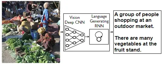
image caption的目标就是根据提供的图像，输出对应的文字描述。如下图所示：

对于图片描述任务，应该尽可能写实，即不需要华丽的语句，只需要陈述图片所展现的事实即可。根据常识，可以知道该任务一般分为两个部分，一是图片编码，二是文本生成，基于此后续的模型也都是encoder-decoder的结构。

人类可以将图像中的视觉信息自动建立关系，进而感知图像的高层语义信息，但是计算机只能提取图像的特征信息，无法向人类大脑一样生成高层语义信息，这就是“语义鸿沟问题”。图像描述技术可以将视觉信息转化为语义信息，有利于解决“语义鸿沟”。

方法

1 传统image caption方法

1.1 基于模板的方法

生成的句子有固定的模板，检测图像中物体、场景和动作等相关元素，在模板中填充相关的词语，组合成句子

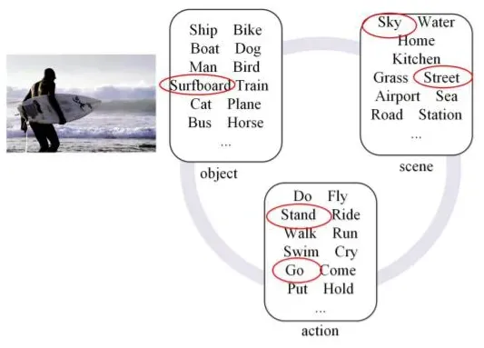
该方法虽然可以生成对图像的准确描述，但是缺点也十分明显，生成的内容单一且较为固定，并且人工参与程度较高。

1.2 基于检索的方法

通过图片匹配的方式实现。先将大量的（图像，图像描述）存入数据库，之后将输入图像与数据库中的图像进行对比，找出相似的图像，将对应的图像描述作为作为候选描述，再对这些描述进行合理的组织，生成输入图像的描述。

这种方法的性能依赖于标注数据集的大小和检索算法，并且受限于相似度计算的准确程度，生成的描述也相对局限，不一定能满足要求。

2 基于深度学习的image caption方法

基于深度学习的方法，概括起来就是有编码器实现对图像的编码，再由解码器生成对应的文字，结合了图像处理和自然语言生成两个方向。

2.1 NIC

论文：Show and Tell: A Neural Image Caption Generator

链接：https://arxiv.org/abs/1411.4555

“show and tell”这篇论文，于2015年提出，首次将深度学习引入image caption任务，提出了encoder-decoder的框架。

作者使用CNN提取图像特征，使用LSTM作为解码器生成对应的图像描述

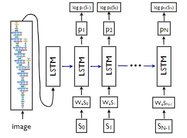
根据上图，有如下计算流程：

式中，表示图像编码，表示将单词进行向量化的参数矩阵，表示图像对应的描述句子，其中表示句子的起始字符，表示句子的结束字符，也就是说，如果有句子there are two books and one pen，那么其应该被处理为<start> there are two books and one pen <end>的形式，当解码器生成<end>时，表示句子生成结束。

使用极大似然估计计算损失函数：

2.2 注意力机制

论文：Show, Attend and Tell: Neural Image Caption Generation with Visual Attention

链接：https://arxiv.org/abs/1502.03044

这篇文章于2015年发布，在NIC的基础上引入了注意力机制，主要对解码器的结构进行改变，其示意图如下：

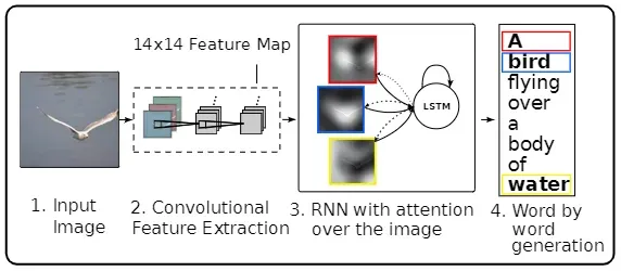
文中，作者一共实验了三种注意力机制，分别为additive attention、stochastic hard attention和deterministic soft attention。

2.2.1 additive attention

注意力权重的计算方式为：

式中,表示注意力权重；表示时间步；表示图像的区域；表示图像区域的向量表示；为LSTM上一个时间步的隐藏层的输出；是注意力模型，由多层MLP实现；表示上下文向量；为一个功能函数，返回单个向量

这里需要注意力得是，前面式子中，注意力模型以多层MLP实现，这是一种叫做“additive attention”的注意力机制。这种方法可以直接看作加权平均，在形式上，给定两组向量：输入向量和隐向量，则和之间的附加注意力计算方式为：

式中，表示激活函数，其代码实现如下：

class Attention(nn.Module):
    """
    Attention Network.
    """

    def __init__(self, encoder_dim, decoder_dim, attention_dim):
        """
        :param encoder_dim: feature size of encoded images
        :param decoder_dim: size of decoder's RNN
        :param attention_dim: size of the attention network
        """
        super(Attention, self).__init__()
        self.encoder_att = nn.Linear(encoder_dim, attention_dim)  # linear layer to transform encoded image
        self.decoder_att = nn.Linear(decoder_dim, attention_dim)  # linear layer to transform decoder's output
        self.full_att = nn.Linear(attention_dim, 1)  # linear layer to calculate values to be softmax-ed
        self.relu = nn.ReLU()
        self.softmax = nn.Softmax(dim=1)  # softmax layer to calculate weights

    def forward(self, encoder_out, decoder_hidden):
        """
        Forward propagation.
        :param encoder_out: encoded images, a tensor of dimension (batch_size, num_pixels, encoder_dim)
        :param decoder_hidden: previous decoder output, a tensor of dimension (batch_size, decoder_dim)
        :return: attention weighted encoding, weights
        """
        att1 = self.encoder_att(encoder_out)  # (batch_size, num_pixels, attention_dim)
        att2 = self.decoder_att(decoder_hidden)  # (batch_size, attention_dim)
        att = self.full_att(self.relu(att1 + att2.unsqueeze(1))).squeeze(2)  # (batch_size, num_pixels)
        alpha = self.softmax(att)  # (batch_size, num_pixels)
        attention_weighted_encoding = (encoder_out * alpha.unsqueeze(2)).sum(dim=1)  # (batch_size, encoder_dim)

        return attention_weighted_encoding, alpha

2.2.2 stochastic hard attention

对于随机注意力机制有：

式中，表示在生成第个单词时，模型会集中注意力的位置变量；表示一种one-hot形式，当区域用于提取视觉特征时置1，否则置0。

模型的目标函数为：

在此注意力机制下，的功能就是，基于由参数化的分布（伯努利）中，在每个时间点采样一个

2.2.3 deterministic soft attention

hard attention需要在每个时间步采样，而soft attention直接使用上下文向量的期望：

接着通过对注释向量加权来确定注意力模型：

这样得到的模型是平滑可微的。

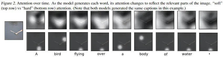
下图为使用soft attention和hard attention的效果对比图：

2.3 其他深度学习网络

2.3.1 review networks

论文：Review Networks for Caption Generation

链接：https://arxiv.org/abs/1605.07912

源码：https://github.com/kimiyoung/review_net

模型结构如下所示：

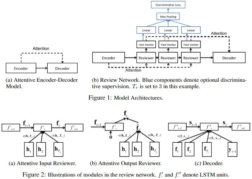
模型的编码器使用的是VGG，解码器使用的是LSTM，比较特别的是，该模型定义了review结构，该结构利用注意力网络对解码器的输入与输出进行了改变。

review包括attentive input reviewer和attentive output reviewer

（1）attentive input reviewer

在每个时间步，使用注意力对隐藏层进行处理，接着用注意力的结果作为解码器中LSTM的输入。有如下公式：

式中，表示注意力输出；表示第个隐层的权重。可以用点积计算，也可以使用多层MLP；表示LSTM单元。

（2）attentive output reviewer

有如下计算公式：

可以看到，与attentive input reviewer的输入不同

（3）Discriminative Supervision

在传统的编码器-解码器模型中，模型的目标是最大化生成序列的条件概率，然而，作者使用了判别性的监督方法，对目标进行预测，如上图蓝色部分所示。简单来说，作者添加了一个损失函数，这个函数有别于生成式模型的损失函数，（或者说，这个损失函数属于判别式模型）。该函数的计算公式如下：

式中，表示归一化因子，表示出现在中所有单词的集合，表示输出，表示单词经过最大池化层后的得分。

模型最后的损失为负的条件对数似然与判别性损失的加权和：

式中，表示输出序列的长度；表示reviewer输出的thought vectors向量集合；表示经过softmax层后的单词的概率；表示第个解码的字符；表示的word embedding。

2.3.2 SCA-CNN

论文：SCA-CNN: Spatial and Channel-wise Attention in Convolutional Networks for Image Captioning

链接：https://arxiv.org/abs/1611.05594

源码：https://github.com/zjuchenlong/sca-cnn.cvpr17

作者认为已有的研究通常使用的是空间注意力（注意力被建模为空间概率，也就是重新加权CNN编码器的最后一个卷积层），这种注意力并不是真正的注意力机制，因此，在CNN中结合了空间和通道注意力。简单来说，作者认为之前使用的注意力不够全面，所以自己在多个不同的地方使用了注意力。

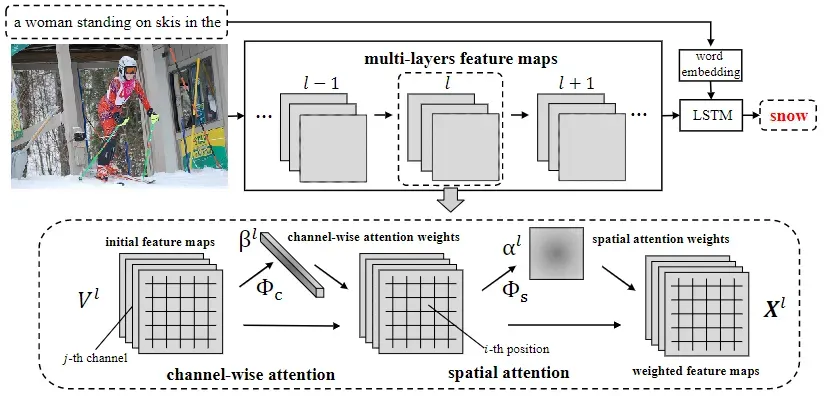
模型的计算流程如下：

式中，表示第层网络层；表示注意力权重；表示注意力函数；表示线性加权函数；表示卷积层的总数。其中注意力权重由空间注意力和通道级注意力组成：

这篇文章的核心为spatial attention和channel wise attention。

（1）spatial attention

空间注意力，也是已有的模型使用的注意力。在已有模型中，仅对编码器最后一个卷积层的feature map使用该注意力机制。在SCA-CNN中，利用了多层卷积提取特征不同的特点，在多层上使用该注意力机制。作者认为，最后一层卷积层的输出已经是后期的输出，也就是说特征基本已经提取完毕，各个像素点之间的差异变小了，注意力机制的效果可能无法有效发挥，而前面网络层的输出，各像素点之间的差异较大，可以更好的发挥注意力机制的效果。

其计算方式为：

式中，表示矩阵与向量相加。

（2）channel wise attention

与空间注意力不同，通道级注意力作用于feature map之间，给每个channel进行加权，所以权重值为向量。作者在编码器网络中，嵌入了这两种注意力机制，并且在多个网络层上进行该操作。

其计算方式为：

式中，表示向量的外积

（3）两种注意力机制的结合方式

作者给出了两种结合方式，channel-spatial和spatial-channel

channel-spatial

通道级注意力在前，空间注意力在后：

spatial-channel

空间注意力在前，通道级注意力在后：

2.3.3 Graph encoder

（1）spatial and semantic graphs
论文：Exploring Visual Relationship for Image Captioning

链接：https://arxiv.org/abs/1809.07041

论文提出了GCN-LSTM模型，使用图卷积网络GCN整合目标之间的语义和空间关系，并将之用于图片编码。

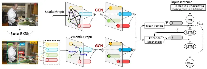
首先使用Faster R-CNN对图像的显著区域进行提取，并构建区域语义有向图（语义图的顶点代表每个区域，边表示每对区域之间的关系）和空间有向图（空间图的顶点表述区域，边表示区域之间的位置关系），以GCN获取embedding输出，再通过带有注意力机制的双层LSTM生成对应的描述。

编码器

原始的GCN使用的是无向图，其计算方式为：

式中，表示激活函数，表示的邻居节点（包括它自己）。

为了使GCN可以融合有向图，并能处理图的标签信息，作者对上式进行了修改：

式中,表示根据每条边的方向选择变换矩阵，如表示，表示，表示。表示每条边的标签。并且，作者给图的每条边加上了门控：

式中，就表示门控。

解码器

解码器使用的注意力机制+双层LSTM的结构。其中，第一层LSTM的参数更新方式为：

式中，表示第二层LSTM的上一个时间步的输出，表示输入单词，表示输入单词对应的转换矩阵，表示经过平均池化后的图像特征。接着根据输出计算注意力权重：

根据注意力得分对图像特征进行加权：

接着合并和，将其作为第二层LSTM的输入：

最后，以作为层的输入，预测下一个单词。

（2）hierarchical trees
论文：Hierarchy Parsing for Image Captioning

链接：https://arxiv.org/abs/1909.03918

该文主要是对编码器进行改进。将图像表示为树形的层次结构，以整体图像作为根节点，中层表示图像的区域，叶节点表示图像区域中的实例对象，接着，将图像树送入TreeLSTM获取图像编码，以提取图像的多层次特征。

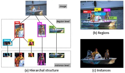
接着，根据图像的层次结构，构建有向图，图的顶点为每个区域或者实例，边表示每对区域或实例之间的关系。

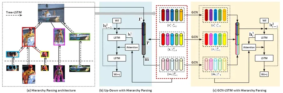
上图为作者提出的层次解析架构（HIP），使用Faster R-CNN检测目标区域，使用Mask R-CNN分割实例集，接着搭建三层的层次树结构，并使用Tree-LSTM自下而上执行，以增强区域和实例特征，并以LSTM实现文本的生成。图的右半部分为作者将HIP结构接入GCN-LSTM模型的示意图。

Tree-LSTM

Tree-LSTM的主要作用就是提取图像的层级特征，其结构如下：

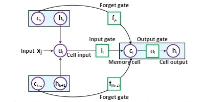
与原始的LSTM不同，Tree-LSTM的状态更新依赖子节点的多个隐藏状态。其状态更新公式如下：

式中，表示当前节点的子集；表示两个向量点积。Tree-LSTM的输入为：

式中，表示区域特征编码，表示实例特征编码

2.3.4 self-attention encoder

（1）Self-Attention

论文：Learning to Collocate Neural Modules for Image Captioning

链接：https://arxiv.org/abs/1904.08608

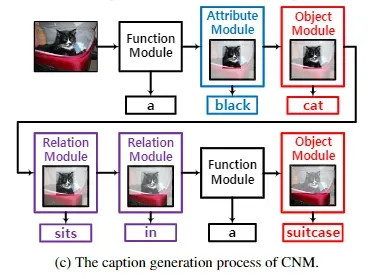
这篇文章的核心就是使用多个网络模块并行（CNM,Collocate Neural Modules）的方式，增强编码器的特征提取能力。不过，值得注意的是，在其中一个模块中，作者使用了多头自注意力。

模型的简要结构如下：

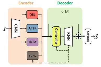
编码器

图中的四个模块分别为object module、attribute module、relation module和function module。

• object module专注于对象类别
• attribute module侧重于视觉属性
• relation module使用了多头自注意力网络，用以学习两个对象之间的交互。其输入为Faster R-CNN提取的ROI特征
• function module用来生成一个功能词，如“a”和“and”

可以结合下图对上述四个模块进行理解：

解码器

解码器使用的了Controller，其结构如下：

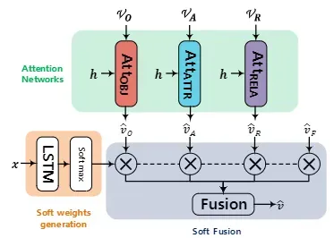
可以看到，该结构包括三个注意力网络和一个LSTM，Controller的输出将会作为后接LSTM的输入，用以生成下一个单词。

其计算流程如下：

1）引入加性注意力机制，将三个视觉模块的输出进行加权

object att:

attribute att:

relation att:

式中表示当前时间步，第一个LSTM的输出。

2）计算soft weight

式中表示第二个LSTM在时刻的输出。

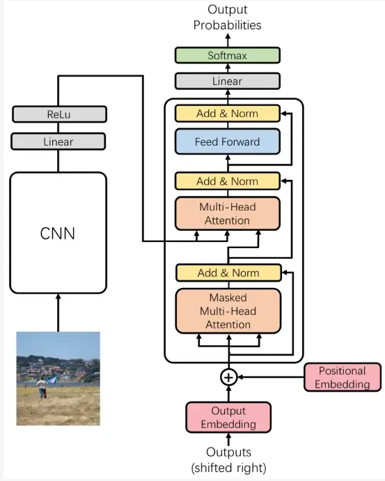
上述文章仅在视觉特征提取方面用了soft-attention的结构，并且该部分特征也只是特征工程的一部分。下面介绍一篇在解码器中使用soft-attention的文章，更确切地说，其使用Transformer的解码器代替了原有的RNN结构的解码器。

论文：Learning to Collocate Neural Modules for Image Captioning

链接：https://arxiv.org/abs/1904.08608

这篇文章的核心就是将原有的RNN结构的解码器用Transformer的解码器替代了，并定义了多级监督机制用以更好的生成当前单词。模型结构如下：

多级监督机制结构如下：

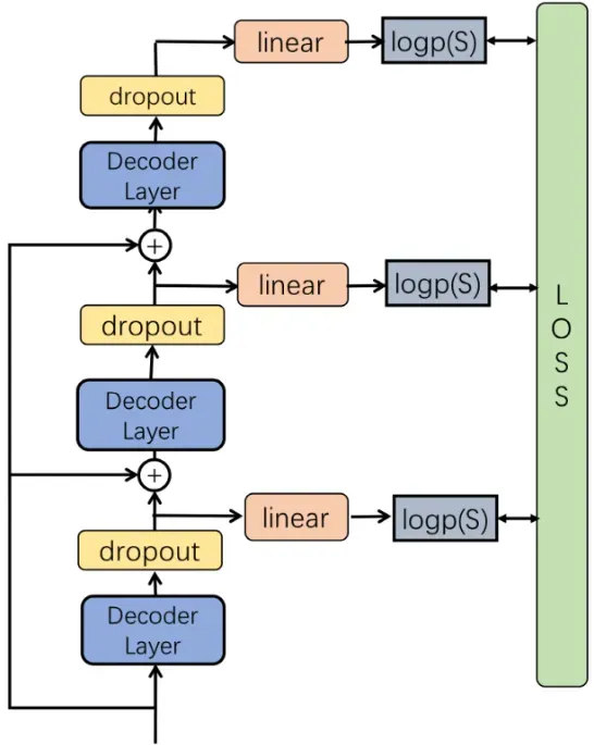
在推理阶段，使用平均池化组合每层的输出，获取单词概率。在训练阶段，使用多输出交叉熵损失：

式中，表示真实句子，表示图像，表示模型参数。

（2）Attention on Attention

论文：Attention on Attention for Image Captioning

链接：https://arxiv.org/abs/1908.06954

源码：https://github.com/husthuaan/AoANet

这篇文章主要是对注意力机制的改进，作者提出了“attention on attention”的方法，该方法通过计算注意力的结果与输入query的相关性来对信息进行过滤，作者最后将该方法运用在编码器和解码器中。

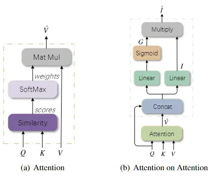
可以看到，AOA中表示“information vector”，表示“attention gate”，最后通过逐元素乘法添加另一个注意力。

将“attention gate”应用于“information vector”：

式中，表示逐元素相乘。作者将这认为是一种注意力，感觉应该是种加性注意力吧。最后，AOA的计算方式如下：

作者在实现AOA的时候也是相对比较简单：

#定义
 if self.use_aoa:
    self.aoa_layer =  nn.Sequential(nn.Linear((1 + scale) * d_model, 2 * d_model), nn.GLU())
    # dropout to the input of AoA layer
    if dropout_aoa > 0:
        self.dropout_aoa = nn.Dropout(p=dropout_aoa)
    else:
        self.dropout_aoa = lambda x:x

if self.use_aoa:
    # Apply AoA
    x = self.aoa_layer(self.dropout_aoa(torch.cat([x, query], -1)))

编码器

编码器结构如下：

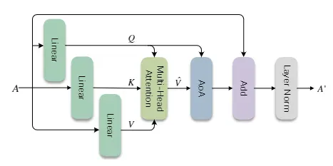
图中和的计算方式如下：

式中，就是多头自注意力机制的计算方式，这里就不再进行赘述；表示CNN输出的图像特征。

可以看到，相比于原始Transformer结构，该编码器增加了AOA结构，并且去掉了前馈网络层，之所以去掉该层作者给出了两个原因：

• 原始结构的前馈网络层是为了增加非线性信息，而本文提出的结构AOA已经满足了这个要求
• 删除前馈网络层并不会影响模型的效果，而且简化了模型的结构

代码实现为：

class AoA_Refiner_Layer(nn.Module):
    def __init__(self, size, self_attn, feed_forward, dropout):
        super(AoA_Refiner_Layer, self).__init__()
        self.self_attn = self_attn
        self.feed_forward = feed_forward
        self.use_ff = 0
        if self.feed_forward is not None:
            self.use_ff = 1
        self.sublayer = clones(SublayerConnection(size, dropout), 1+self.use_ff)
        self.size = size

    def forward(self, x, mask):
        x = self.sublayer[0](x, lambda x: self.self_attn(x, x, x, mask))
        return self.sublayer[-1](x, self.feed_forward) if self.use_ff else x

class AoA_Refiner_Core(nn.Module):
    def __init__(self, opt):
        super(AoA_Refiner_Core, self).__init__()
        attn = MultiHeadedDotAttention(opt.num_heads, opt.rnn_size, project_k_v=1, scale=opt.multi_head_scale, do_aoa=opt.refine_aoa, norm_q=0, dropout_aoa=getattr(opt, 'dropout_aoa', 0.3))
        layer = AoA_Refiner_Layer(opt.rnn_size, attn, PositionwiseFeedForward(opt.rnn_size, 2048, 0.1) if opt.use_ff else None, 0.1)
        self.layers = clones(layer, 6)
        self.norm = LayerNorm(layer.size)
        
    def forward(self, x, mask):
        for layer in self.layers:
            x = layer(x, mask)
        return self.norm(x)

解码器

解码器的结构如下：

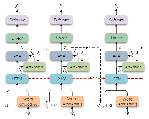
作者对上下文向量建模，计算词语的条件概率：

保存着解码状态和新获取的信息，由编码器输出的和LSTM输出的生成。LSTM的输入为输入单词的向量表征、上下文向量和编码暗器的输出：

式中，在时间步下，输入单词的One-hot编码。

代码实现如下：

class AoA_Decoder_Core(nn.Module):
    def __init__(self, opt):
        super(AoA_Decoder_Core, self).__init__()
        self.drop_prob_lm = opt.drop_prob_lm
        self.d_model = opt.rnn_size
        self.use_multi_head = opt.use_multi_head
        self.multi_head_scale = opt.multi_head_scale
        self.use_ctx_drop = getattr(opt, 'ctx_drop', 0)
        self.out_res = getattr(opt, 'out_res', 0)
        self.decoder_type = getattr(opt, 'decoder_type', 'AoA')
        self.att_lstm = nn.LSTMCell(opt.input_encoding_size + opt.rnn_size, opt.rnn_size) # we, fc, h^2_t-1
        self.out_drop = nn.Dropout(self.drop_prob_lm)

        if self.decoder_type == 'AoA':
            # AoA layer
            self.att2ctx = nn.Sequential(nn.Linear(self.d_model * opt.multi_head_scale + opt.rnn_size, 2 * opt.rnn_size), nn.GLU())
        elif self.decoder_type == 'LSTM':
            # LSTM layer
            self.att2ctx = nn.LSTMCell(self.d_model * opt.multi_head_scale + opt.rnn_size, opt.rnn_size)
        else:
            # Base linear layer
            self.att2ctx = nn.Sequential(nn.Linear(self.d_model * opt.multi_head_scale + opt.rnn_size, opt.rnn_size), nn.ReLU())

        # if opt.use_multi_head == 1: # TODO, not implemented for now           
        #     self.attention = MultiHeadedAddAttention(opt.num_heads, opt.d_model, scale=opt.multi_head_scale)
        if opt.use_multi_head == 2:            
            self.attention = MultiHeadedDotAttention(opt.num_heads, opt.rnn_size, project_k_v=0, scale=opt.multi_head_scale, use_output_layer=0, do_aoa=0, norm_q=1)
        else:            
            self.attention = Attention(opt)

        if self.use_ctx_drop:
            self.ctx_drop = nn.Dropout(self.drop_prob_lm)        
        else:
            self.ctx_drop = lambda x :x

    def forward(self, xt, mean_feats, att_feats, p_att_feats, state, att_masks=None):
        # state[0][1] is the context vector at the last step
        h_att, c_att = self.att_lstm(torch.cat([xt, mean_feats + self.ctx_drop(state[0][1])], 1), (state[0][0], state[1][0]))

        if self.use_multi_head == 2:
            att = self.attention(h_att, p_att_feats.narrow(2, 0, self.multi_head_scale * self.d_model), p_att_feats.narrow(2, self.multi_head_scale * self.d_model, self.multi_head_scale * self.d_model), att_masks)
        else:
            att = self.attention(h_att, att_feats, p_att_feats, att_masks)

        ctx_input = torch.cat([att, h_att], 1)
        if self.decoder_type == 'LSTM':
            output, c_logic = self.att2ctx(ctx_input, (state[0][1], state[1][1]))
            state = (torch.stack((h_att, output)), torch.stack((c_att, c_logic)))
        else:
            output = self.att2ctx(ctx_input)
            # save the context vector to state[0][1]
            state = (torch.stack((h_att, output)), torch.stack((c_att, state[1][1])))

        if self.out_res:
            # add residual connection
            output = output + h_att

        output = self.out_drop(output)
        return output, state

（3）Geometry-Aware Self-Attention

论文：Captioning Transformer with Stacked Attention Modules

链接：https://www.mdpi.com/2076-3417/8/5/739

在这篇文章中，作者提出了“归一化的自注意力（NSA）”和“Geometry-aware self-attention（GSA）”。简单来说，作者有两个创新点，一是自定义了一种归一化的方法用以代替layer normalization（LN），并提出了一种适用于图像的位置信息表示方法，将该方法用于自注意力机制中。

self-attention network(SAN)

注意力网络用于图像描述的一般范式如下：

一般模型会遵循Transformer的结构，使用编码器对图像编码，使用解码器生成文本。作者的模型整体结构与SAN相似，不过其在归一化和位置信息上做了改变。

NSA

原始的soft-attention的计算方式为：

作者给出的计算方式为：

可以看到，作者以一个全连接层代替了原有的矩阵乘积的方式。

GSA

针对图像区域的特点，引入区域的位置信息，其表示方式如下：

式中，表示图像区域中心坐标；表示区域的宽；表示区域的高。

接着使用全连接层将映射到高维向量表征：

将的信息加入到注意力得分中：

式中，表示几何注意力函数；是几何注意力机制的查询和键，其计算方式与自注意力一致。对于有三种选择：

• Content-independent:
• Query-dependent:
• Key-dependent:

作者在实验时，NSA并未用于解码器中，因为解码器是自回归模型，其长度可变的性质不适合。

3 基于预训练模型的image caption方法

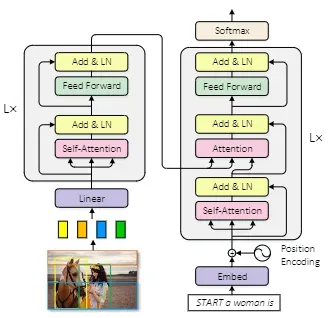
3.1 VLP

论文：Unified Vision-Language Pre-Training for Image Captioning and VQA

链接：https://arxiv.org/abs/1909.11059

源码：https://github.com/LuoweiZhou/VLP

该文章提出的模型既可以完成生成式任务，又可以完成理解式任务，并且使用共享的多层Transformer层进行编码和解码。VLP在大量的图文对上进行预训练，训练任务为“image caption”和“visual question answer”。模型的训练方式如下图所示：

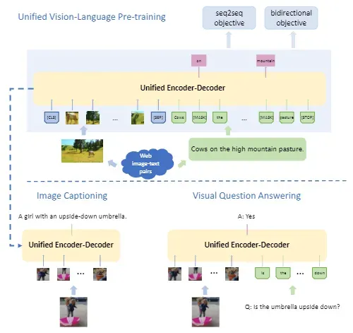
可以看到，在预训练阶段，图像信息在文本信息的前面。

模型的结构如下图所示：

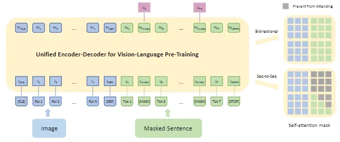
可以看到模型的输入为：region embedding、word embedding和三个特殊toekn。

图文embedding编码合并的代码实现：

if vis_input:
    words_embeddings = torch.cat((words_embeddings[:, :1], vis_feats,
        words_embeddings[:, len_vis_input+1:]), dim=1)
    assert len_vis_input == 100, 'only support region attn!'
    position_embeddings = torch.cat((position_embeddings[:, :1], vis_pe,
        position_embeddings[:, len_vis_input+1:]), dim=1) # hacky...

模型的结构与BERT一致，都是12层的Transformer层，不同之处就是输入和训练任务了。

3.2 BLIP

论文：BLIP: Bootstrapping Language-Image Pre-training for Unified Vision-Language Understanding and Generation

链接：https://arxiv.org/abs/2201.12086

源码：https://github.com/salesforce/BLIP

作者分析了已有的模型在模型结构和数据来源的不足，做出了两个贡献。1）提出了一种编码器-解码器的多模式混合结构，可以有效的进行多任务的预训练和迁移学习；2）提出了一种bootstrapping方法，用以处理数据集，这是一种数据增强的方法。BLIP在零样本或小样本学习上表现十分不错。

（1）模型方面

BLIP模型结构如下：

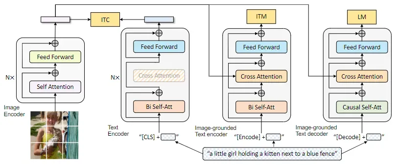
图中，相同颜色模块具有相同的参数。可以看到，模型可以分为三个板块，其中ITC表示“image-text contrative”，用来对齐视觉和语言表示；ITM表示“image-text matching”，使用交叉注意力层来模拟图文信息交互，来区分正负图像-文本对；LM表示“language model”，用causal注意力代替双向注意力机制，并且与编码器共享参数，用来生成图片描述。作者将这种结构称作MED(multimodal mixture of encoder-decoder)。

模型可以运行符合unimodal encoder、image-grounded text encoder和image-grounded text decoder三种形式的任务。

unimodal encoder

图像和文本编码，文本编码器与BERT一致，字符“[CLS]”用作文本编码表示。

代码实现如下：

image_embeds = self.visual_encoder(image) 
image_atts = torch.ones(image_embeds.size()[:-1],dtype=torch.long).to(image.device)        
image_feat = F.normalize(self.vision_proj(image_embeds[:,0,:]),dim=-1)          

text = self.tokenizer(caption, padding='max_length', truncation=True, max_length=30, 
                    return_tensors="pt").to(image.device)  
text_output = self.text_encoder(text.input_ids, attention_mask = text.attention_mask,                      
                              return_dict = True, mode = 'text')            
text_feat = F.normalize(self.text_proj(text_output.last_hidden_state[:,0,:]),dim=-1)                 

# get momentum features
with torch.no_grad():
  self._momentum_update()
  image_embeds_m = self.visual_encoder_m(image) 
  image_feat_m = F.normalize(self.vision_proj_m(image_embeds_m[:,0,:]),dim=-1)  
  image_feat_all = torch.cat([image_feat_m.t(),self.image_queue.clone().detach()],dim=1)                   

  text_output_m = self.text_encoder_m(text.input_ids, attention_mask = text.attention_mask,                      
                                      return_dict = True, mode = 'text')    
  text_feat_m = F.normalize(self.text_proj_m(text_output_m.last_hidden_state[:,0,:]),dim=-1) 
  text_feat_all = torch.cat([text_feat_m.t(),self.text_queue.clone().detach()],dim=1)

  sim_i2t_m = image_feat_m @ text_feat_all / self.temp  
  sim_t2i_m = text_feat_m @ image_feat_all / self.temp 

  sim_targets = torch.zeros(sim_i2t_m.size()).to(image.device)
  sim_targets.fill_diagonal_(1)          

  sim_i2t_targets = alpha * F.softmax(sim_i2t_m, dim=1) + (1 - alpha) * sim_targets
  sim_t2i_targets = alpha * F.softmax(sim_t2i_m, dim=1) + (1 - alpha) * sim_targets        

sim_i2t = image_feat @ text_feat_all / self.temp
sim_t2i = text_feat @ image_feat_all / self.temp

loss_i2t = -torch.sum(F.log_softmax(sim_i2t, dim=1)*sim_i2t_targets,dim=1).mean()
loss_t2i = -torch.sum(F.log_softmax(sim_t2i, dim=1)*sim_t2i_targets,dim=1).mean() 

loss_ita = (loss_i2t+loss_t2i)/2

image-grounded text encoder

在双向自注意力和前馈网络层之间插入了交叉注意力，用作图文特征的交互。并定义了特殊字符“[Encode]”，放置在文本开头，用作多模态表示。

代码实现如下：

encoder_input_ids = text.input_ids.clone()
encoder_input_ids[:,0] = self.tokenizer.enc_token_id

# forward the positve image-text pair
bs = image.size(0)
output_pos = self.text_encoder(encoder_input_ids,
                               attention_mask = text.attention_mask,
                               encoder_hidden_states = image_embeds,
                               encoder_attention_mask = image_atts,      
                               return_dict = True,
                              )            
with torch.no_grad():       
    weights_t2i = F.softmax(sim_t2i[:,:bs],dim=1)+1e-4 
    weights_t2i.fill_diagonal_(0)            
    weights_i2t = F.softmax(sim_i2t[:,:bs],dim=1)+1e-4  
    weights_i2t.fill_diagonal_(0)   

# select a negative image for each text
image_embeds_neg = []    
for b in range(bs):
    neg_idx = torch.multinomial(weights_t2i[b], 1).item()
    image_embeds_neg.append(image_embeds[neg_idx])
image_embeds_neg = torch.stack(image_embeds_neg,dim=0)   

# select a negative text for each image
text_ids_neg = []
text_atts_neg = []
for b in range(bs):
    neg_idx = torch.multinomial(weights_i2t[b], 1).item()
    text_ids_neg.append(encoder_input_ids[neg_idx])
    text_atts_neg.append(text.attention_mask[neg_idx])

text_ids_neg = torch.stack(text_ids_neg,dim=0)   
text_atts_neg = torch.stack(text_atts_neg,dim=0)      

text_ids_all = torch.cat([encoder_input_ids, text_ids_neg],dim=0)     
text_atts_all = torch.cat([text.attention_mask, text_atts_neg],dim=0)     

image_embeds_all = torch.cat([image_embeds_neg,image_embeds],dim=0)
image_atts_all = torch.cat([image_atts,image_atts],dim=0)

output_neg = self.text_encoder(text_ids_all,
                               attention_mask = text_atts_all,
                               encoder_hidden_states = image_embeds_all,
                               encoder_attention_mask = image_atts_all,      
                               return_dict = True,
                              )                            

vl_embeddings = torch.cat([output_pos.last_hidden_state[:,0,:], output_neg.last_hidden_state[:,0,:]],dim=0)
vl_output = self.itm_head(vl_embeddings)            

itm_labels = torch.cat([torch.ones(bs,dtype=torch.long),torch.zeros(2*bs,dtype=torch.long)],
                       dim=0).to(image.device)
loss_itm = F.cross_entropy(vl_output, itm_labels) 

image-grounded text decoder

用因果自注意力层替换双向自注意力层，增加了特殊字符“[Decode]”，用于表示序列的开始，序列结束标记依旧用“end”表示。

代码实现如下：

decoder_input_ids = text.input_ids.clone()      
decoder_input_ids[:,0] = self.tokenizer.bos_token_id
decoder_targets = decoder_input_ids.masked_fill(decoder_input_ids == self.tokenizer.pad_token_id, -100) 

decoder_output = self.text_decoder(decoder_input_ids, 
                                   attention_mask = text.attention_mask, 
                                   encoder_hidden_states = image_embeds,
                                   encoder_attention_mask = image_atts,                  
                                   labels = decoder_targets,
                                   return_dict = True,   
                                  )   

loss_lm = decoder_output.loss  

最后，作者结合上述三个模块实现整体的MED结构。

其交叉注意力和因果注意力的实现代码为：

  if is_cross_attention:
      key_layer = self.transpose_for_scores(self.key(encoder_hidden_states))
      value_layer = self.transpose_for_scores(self.value(encoder_hidden_states))
      attention_mask = encoder_attention_mask
  elif past_key_value is not None:
      key_layer = self.transpose_for_scores(self.key(hidden_states))
      value_layer = self.transpose_for_scores(self.value(hidden_states))
      key_layer = torch.cat([past_key_value[0], key_layer], dim=2)
      value_layer = torch.cat([past_key_value[1], value_layer], dim=2)
  else:
      key_layer = self.transpose_for_scores(self.key(hidden_states))
      value_layer = self.transpose_for_scores(self.value(hidden_states))

其中，past_key_value部分就是因果注意力的实现，单说注意力部分，作者通过对key和value的不同定义，来实现交叉注意力和因果注意力。在交叉注意力中，key和value使用来自编码器的输出，在其他注意力中使用来自文本的hidden states。

编码器部分，图片使用的是VIT模型，文本使用的是BERT：

self.visual_encoder, vision_width = create_vit(vit,image_size, vit_grad_ckpt, vit_ckpt_layer)
self.text_encoder = BertModel(config=med_config, add_pooling_layer=False)  

（2）数据方面

数据的处理流程如下图所示：

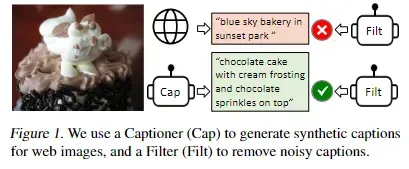
针对网络上的劣质文本数据，作者使用模型生成图片对应的文本描述，并使用过滤器过滤噪声数据，合并两者的结果，形成高质量的图片-文本数据对。

BLIP模型预训练和数据增强的原理如下：

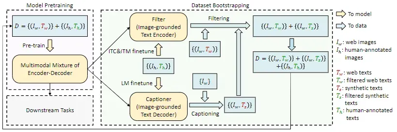
数据处理部分主要有两个模块，captioning（用于生成给定图像的文字描述）和filtering（用于去除噪声图像文本对），两者均以MED进行初始化，并在数据集COCO上微调。最后合并两者的数据集，以新的数据集预训练一个新的模型。

3.3 OFA

论文：OFA: Unifying Architectures, Tasks, and Modalities Through a Simple Sequence-to-Sequence Learning Frameworkon

链接：https://arxiv.org/abs/2202.03052

源码：https://github.com/OFA-Sys/OFA

OFA是阿里巴巴提出的模型，寓意“one for all”，模型统一了多种视觉和语言，理解和生成任务。其预训练任务如下图所示：

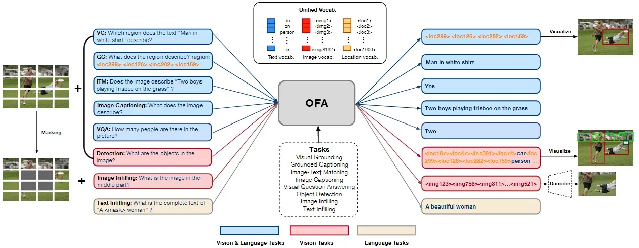
大致包括区域检测、区域字幕、图文匹配、图像字幕、视觉问答、目标检测、图像填充和文本填充。（部分任务名称描述可能不够专业，因为没做过多了解）

模型使用encoder-decoder的架构，并依旧以Transformer为基础实现。由于论文大部分内容展示的是实验，所以可展开的内容较少。

实验

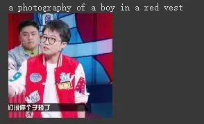
终于到了令人激动的实验环节。本文实验不对模型进行微调，仅展示模型BLIP和OFA的使用方法。

1 BLIP

代码如下：

import requests
from PIL import Image
from transformers import BlipProcessor, BlipForConditionalGeneration

processor = BlipProcessor.from_pretrained("Salesforce/blip-image-captioning-base")
model = BlipForConditionalGeneration.from_pretrained("Salesforce/blip-image-captioning-base").to("cuda")

# img_url = 'https://storage.googleapis.com/sfr-vision-language-research/BLIP/demo.jpg' 
img_url = 'https://ww4.sinaimg.cn/thumb150/006ymYXKgy1gahftdd597j31o00u079k.jpg'
raw_image = Image.open(requests.get(img_url, stream=True).raw).convert('RGB')

# conditional image captioning
text = "a photography of"
inputs = processor(raw_image, text, return_tensors="pt").to("cuda")

out = model.generate(**inputs)
print(processor.decode(out[0], skip_special_tokens=True))

# unconditional image captioning
# inputs = processor(raw_image, return_tensors="pt").to("cuda")

# out = model.generate(**inputs)
# print(processor.decode(out[0], skip_special_tokens=True))

零样本下的结果：

2 OFA

代码如下：

!git clone --single-branch --branch feature/add_transformers https://github.com/OFA-Sys/OFA.git
!pip install OFA/transformers/
!git clone https://huggingface.co/OFA-Sys/OFA-tiny


from PIL import Image
from torchvision import transforms
from transformers import OFATokenizer, OFAModel
from transformers.models.ofa.generate import sequence_generator
import requests
import torch

mean, std = [0.5, 0.5, 0.5], [0.5, 0.5, 0.5]
resolution = 480
patch_resize_transform = transforms.Compose([
        lambda image: image.convert("RGB"),
        transforms.Resize((resolution, resolution), interpolation=Image.BICUBIC),
        transforms.ToTensor(), 
        transforms.Normalize(mean=mean, std=std)
    ])

ckpt_dir="OFA-Sys/ofa-large-caption"
tokenizer = OFATokenizer.from_pretrained(ckpt_dir)

txt = " what does the image describe?"
inputs = tokenizer([txt], return_tensors="pt").input_ids
url='https://ww4.sinaimg.cn/thumb150/006ymYXKgy1gahftdd597j31o00u079k.jpg'
img=Image.open(requests.get(url,stream=True).raw)
print(img)
patch_img = patch_resize_transform(img).unsqueeze(0)


# using the generator of fairseq version
model = OFAModel.from_pretrained(ckpt_dir, use_cache=True)
generator = sequence_generator.SequenceGenerator(
                    tokenizer=tokenizer,
                    beam_size=5,
                    max_len_b=16, 
                    min_len=0,
                    no_repeat_ngram_size=3,
                )
data = {}
data["net_input"] = {"input_ids": inputs, 'patch_images': patch_img, 'patch_masks':torch.tensor([True])}
gen_output = generator.generate([model], data)
gen = [gen_output[i][0]["tokens"] for i in range(len(gen_output))]

# using the generator of huggingface version
model = OFAModel.from_pretrained(ckpt_dir, use_cache=False)
gen = model.generate(inputs, patch_images=patch_img, num_beams=5, no_repeat_ngram_size=3) 

print(tokenizer.batch_decode(gen, skip_special_tokens=True))

零样本下的结果：

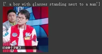
对比两个模型生成的描述：

BLIP: a photography of a boy in a red vest

OFA: a boy with glasses standing next to a man

根据两个模型的结果，我们也不能说谁好谁坏，在我看来，将两者的结果结合可能才是最佳的。

同时，可以发现BLIP和OFA还是有较大差别的，单从这一个例子可以看出，BLIP可以对图像中的视觉信息进行更好的描述（如红色衣服），OFA更注重对图片中的实例信息的描述（如描述了两个人之间的位置关系，描述了戴着眼镜）。换言之，BLIP对视觉特征的提取更好，OFA对实例特征的提取更好。当然，这也与模型的训练数据有关。想进一步了解的同学，可以使用更多的数据集进行对比。

总结

本文围绕image caption，以论文介绍的形式，说明了如何实现image caption。从传统方法、深度学习方法和基于预训练模型的方法，三个方面对已有的研究方法进行了说明。其中传统方法包括：基于模板和基于检索的方法。深度学习方法包括：第一篇论文NIC方法、基于注意力机制的方法、基于图神经的方法、基于自注意力的方法以及其他深度学习方法。基于预训练模型的方法包括：VLP、BLIP和OFA。在介绍完已有方法后，对BLIP和OFA进行了零样本实验。

根据上述方法，可以将其创新点概括为以下几个方面：

• 编码器

  • 使用多种网络提取多方面的视觉特征
  • 图像层次特征的提取

• 解码器

  • 引入注意力机制
  • 注意力机制的结构
  • 二维位置信息提取

• 预训练模型

  • 如何实现多模态交互

本文的不足之处：未对基于对抗网络的方法进行介绍，未对基于强化学习的方法进行介绍，未对代码进行讲解等等。

【参考文章】

1、chrome-extension://bocbaocobfecmglnmeaeppambideimao/pdf/viewer.html?file=http%3A%2F%2Fwww.nlpir.org%2Fwordpress%2Fwp-content%2Fuploads%2F2021%2F10%2FImage_Caption.pdf

2、https://aitechtogether.com/article/12841.html

3、http://html.rhhz.net/tis/html/201910039.htm

4、https://zhuanlan.zhihu.com/p/358127578

5、https://www.yanxishe.com/blogDetail/28479