文章目录
- 前言
- 1. 算法结合思路
- 2. 问题场景
- 2.1 Sphere
- 2.2 Himmelblau
- 2.3 Ackley
- 2.4 函数可视化
- 3. 算法实现
- 代码仓库:IALib[GitHub]
前言
本篇是智能算法(Python复现)专栏的第四篇文章,主要介绍粒子群优化算法与模拟退火算法的结合,以弥补各自算法之间的不足。
在上篇博客【智能算法系列之粒子群优化算法】中有介绍到混合粒子群优化算法,比如将粒子更新后所获得的新的粒子,采用模拟退火的思想决定是否接受进入下一代迭代。不过啊,本篇也算是混合粒子群优化算法吧,侧重点是将粒子群优化应用在模拟退火算法中,而不是在粒子群优化算法中应用模拟退火算法。
1. 算法结合思路
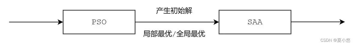
在这篇博客【智能算法系列之模拟退火算法】中介绍到的模拟退火算法有可以优化的地方,比如在初始解得选择上,默认是随机选择一个解作为初始解,所以想法就来了:如果初始解是一个局部最优解,在此基础之上应用模拟退火算法,那结果肯定会比随机初始解效果好。
如何选择这个初始解或者局部最优解呢,那又有很多算法了,前面介绍的遗传算法和粒子群优化算法都可以使用,本篇就使用粒子群优化来选择初始解。
后续也会在本篇中更新使用遗传算法来选择初始解,不过不打算更新此算法的文章,详细的可以查阅 IALib 库代码。
正如上述所说,本篇并没有在每一代中都应用模拟退火算法(这样的话就是混合粒子群了),而是这样:
2. 问题场景
依然是最值问题,不过将原始的一元函数最值问题换成了二元函数最值问题[复杂度也没增加多少,主要是为了方便可视化]。本次求解三个经典函数的最值:
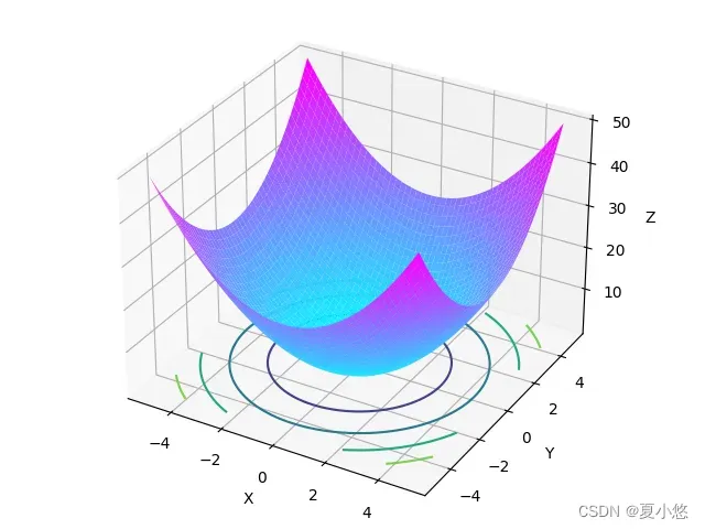
2.1 Sphere
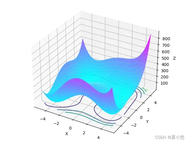
2.2 Himmelblau
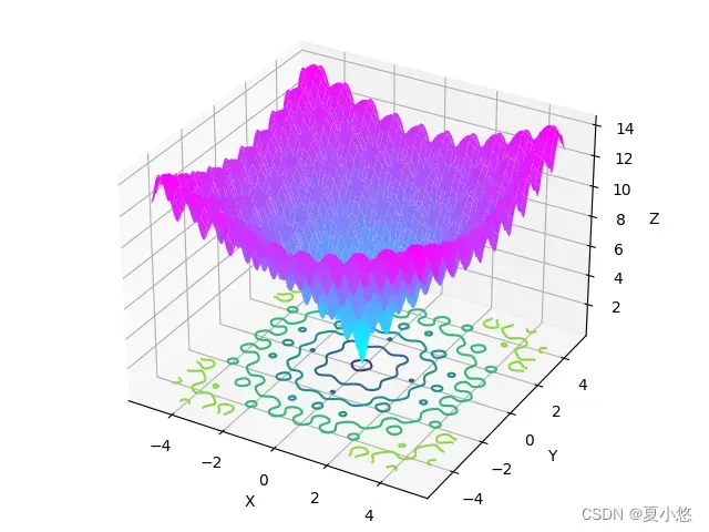
2.3 Ackley
其中,
.
2.4 函数可视化
# -*- coding:utf-8 -*-
# Author:   xiayouran
# Email:    youran.xia@foxmail.com
# Datetime: 2023/3/30 14:22
# Filename: visu_func.py
import numpy as np
import matplotlib.pyplot as plt
from mpl_toolkits.mplot3d import Axes3D


class Visu3DFunc(object):
    def __init__(self, func_name='Sphere'):
        self.func_name = func_name
        self.X = np.linspace(-5, 5, num=200)
        self.Y = np.linspace(-5, 5, num=200)

    @classmethod
    def sphere(cls, x, y):
        """Sphere"""
        return x**2 + y**2

    @classmethod
    def himmelblau(cls, x, y):
        """Himmelblau"""
        return (x**2 + y - 11)**2 + (x + y**2 - 7)**2

    @classmethod
    def ackley(cls, x, y, a=20, b=0.2, c=2*np.pi):
        """Ackley"""
        term1 = -a * np.exp(-b * np.sqrt((x**2 + y**2)/2))
        term2 = -np.exp((np.cos(c*x) + np.cos(c*y))/2)
        return term1 + term2 + a + np.exp(1)

    def draw(self):
        fig = plt.figure()
        # ax = fig.gca(projection='3d')
        ax = Axes3D(fig)
        X, Y = np.meshgrid(self.X, self.Y)

        if self.func_name == 'Sphere':
            Z = self.sphere(X, Y)
        elif self.func_name == 'Himmelblau':
            Z = self.himmelblau(X, Y)
        else:
            Z = self.ackley(X, Y)

        ax.plot_surface(X, Y, Z, cmap=plt.cm.cool)
        ax.contour(X, Y, Z, levels=5, offset=0)
        ax.set_xlabel('X')
        ax.set_ylabel('Y')
        ax.set_zlabel('Z')
        ax.set_title('{} Function'.format(self.func_name))
        # ax.scatter3D(0, 0, self.sphere(0, 0), s=100, lw=0, c='green', alpha=0.7)
        plt.savefig(self.func_name)

        plt.show()


if __name__ == '__main__':
    # Sphere, Himmelblau, Ackley
    visu_obj = Visu3DFunc(func_name='Sphere')
    visu_obj.draw()
3. 算法实现
# -*- coding:utf-8 -*-
# Author:   xiayouran
# Email:    youran.xia@foxmail.com
# Datetime: 2023/3/30 15:50
# Filename: pso_saa.py
import numpy as np
import matplotlib.pyplot as plt
from mpl_toolkits.mplot3d import Axes3D

from IALib.base_algorithm import BaseAlgorithm
from IALib.particle_swarm_optimization import ParticleSwarmOptimization, Particle
from IALib.simulate_anneal_algorithm import SimulateAnnealAlgorithm
from IALib.mixup.visu_func import Visu3DFunc


__all__ = ['PSO_SAA']


class PSO_SAA(BaseAlgorithm):
    def __init__(self, population_size=100, p_dim=1, v_dim=1, max_iter=500, x_range=(0, 5),
                 t_max=1.0, t_min=1e-3, coldrate=0.9, seed=10086):
        super(PSO_SAA, self).__init__()
        self.__population_size = population_size  # 种群大小
        self.__p_dim = p_dim        # 粒子位置维度
        self.__v_dim = v_dim        # 粒子速度维度
        self.__max_iter = max_iter  # 最大迭代次数
        self.__t_max = t_max  # 初始温度
        self.__t_min = t_min  # 终止温度
        self.__coldrate = coldrate  # 降温速率
        self.saa_best_particle = None   # 模拟退火算法得到的最优解
        self.best_particle = None       # 最优解
        self.__x_range = x_range
        self.__seed = seed
        self.optimal_solution = None

        np.random.seed(self.__seed)

    def problem_function(self, x):
        if self.__p_dim == 1:
            return super().problem_function(x)
        else:
            return Visu3DFunc.sphere(*x)

    def solution(self):
        # PSO
        algo_pso = ParticleSwarmOptimization(population_size=self.__population_size,
                                             p_dim=self.__p_dim, v_dim=self.__v_dim,
                                             max_iter=self.__max_iter, x_range=self.__x_range)
        algo_pso.solution()

        # SAA
        x = algo_pso.global_best_particle.best_position   # 初始解
        while self.__t_max > self.__t_min:
            for _ in range(self.__max_iter):
                x_new = np.clip(x + np.random.randn(), a_min=self.__x_range[0], a_max=self.__x_range[1])
                delta = self.problem_function(x_new) - self.problem_function(x)  # 计算目标函数的值差
                if delta < 0:  # 局部最优解
                    x = x_new   # 直接接受更优解
                else:
                    p = np.exp(-delta / self.__t_max)  # 粒子在温度T时趋于平衡的概率为exp[-ΔE/(kT)]
                    r = np.random.uniform(0, 1)
                    if p > r:  # 以一定概率来接受最优解
                        x = x_new
            self.__t_max *= self.__coldrate

        # optimal solution
        saa_best_particle = Particle()
        saa_best_particle.position = x
        saa_best_particle.best_position = x
        saa_best_particle.fitness = self.problem_function(x)
        self.saa_best_particle = saa_best_particle

        if saa_best_particle.fitness < algo_pso.global_best_particle.fitness:
            self.best_particle = saa_best_particle
        else:
            self.best_particle = algo_pso.global_best_particle

        self.optimal_solution = (self.parse_format(self.best_particle.position),
                                 self.parse_format(self.best_particle.fitness))
        print('the optimal solution is', self.optimal_solution)
        # print('optimal solution:\nposition: {} \nfitness: {}'.format(self.best_particle.best_position,
        #                                                              self.best_particle.fitness))

    def draw(self):
        # PSO
        algo_pso = ParticleSwarmOptimization(population_size=self.__population_size,
                                             p_dim=self.__p_dim, v_dim=self.__v_dim,
                                             max_iter=self.__max_iter, x_range=self.__x_range)
        algo_pso.draw(mixup=True)
        plt.clf()
        x = np.linspace(*self.__x_range, 200)
        plt.plot(x, self.problem_function(x))

        # SAA
        x = algo_pso.global_best_particle.best_position   # 初始解
        while self.__t_max > self.__t_min:
            for _ in range(self.__max_iter):
                # something about plotting
                if 'sca' in globals() or 'sca' in locals():
                    sca.remove()
                sca = plt.scatter(x, self.problem_function(x), s=100, lw=0, c='red', alpha=0.5)
                plt.pause(0.01)

                x_new = np.clip(x + np.random.randn(), a_min=self.__x_range[0], a_max=self.__x_range[1])
                delta = self.problem_function(x_new) - self.problem_function(x)  # 计算目标函数的值差
                if delta < 0:  # 局部最优解
                    x = x_new   # 直接接受更优解
                else:
                    p = np.exp(-delta / self.__t_max)  # 粒子在温度T时趋于平衡的概率为exp[-ΔE/(kT)]
                    r = np.random.uniform(0, 1)
                    if p > r:  # 以一定概率来接受最优解
                        x = x_new
            self.__t_max *= self.__coldrate

        # optimal solution
        saa_best_particle = Particle()
        saa_best_particle.position = x
        saa_best_particle.best_position = x
        saa_best_particle.fitness = self.problem_function(x)
        self.saa_best_particle = saa_best_particle

        if saa_best_particle.fitness < algo_pso.global_best_particle.fitness:
            self.best_particle = saa_best_particle
        else:
            self.best_particle = algo_pso.global_best_particle

        plt.scatter(self.best_particle.best_position, self.best_particle.fitness, s=100, lw=0, c='green', alpha=0.7)
        plt.ioff()
        plt.show()

        self.optimal_solution = (self.parse_format(self.best_particle.position),
                                 self.parse_format(self.best_particle.fitness))
        print('the optimal solution is', self.optimal_solution)
        # print('optimal solution:\nposition: {} \nfitness: {}'.format(self.best_particle.best_position,
        #                                                              self.best_particle.fitness))

    def draw3D(self):
        # PSO
        algo_pso = ParticleSwarmOptimization(population_size=self.__population_size,
                                             p_dim=self.__p_dim, v_dim=self.__v_dim,
                                             max_iter=self.__max_iter, x_range=self.__x_range)
        algo_pso.draw3D(mixup=True)
        plt.clf()
        ax = Axes3D(algo_pso.fig)
        x_ = np.linspace(*self.__x_range, num=200)
        X, Y = np.meshgrid(x_, x_)
        Z = self.problem_function([X, Y])
        ax.plot_surface(X, Y, Z, cmap=plt.cm.cool)
        ax.contour(X, Y, Z, levels=5, offset=0)
        ax.set_xlabel('X')
        ax.set_ylabel('Y')
        ax.set_zlabel('Z')

        # SAA
        x = algo_pso.global_best_particle.best_position   # 初始解
        while self.__t_max > self.__t_min:
            for _ in range(self.__max_iter):
                # something about plotting
                if 'sca' in globals() or 'sca' in locals():
                    sca.remove()
                sca = ax.scatter3D(*x, self.problem_function(x), s=100, lw=0, c='red', alpha=0.5)
                plt.pause(0.01)

                x_new = np.clip(x + np.random.randn(), a_min=self.__x_range[0], a_max=self.__x_range[1])
                delta = self.problem_function(x_new) - self.problem_function(x)  # 计算目标函数的值差
                if delta < 0:  # 局部最优解
                    x = x_new   # 直接接受更优解
                else:
                    p = np.exp(-delta / self.__t_max)  # 粒子在温度T时趋于平衡的概率为exp[-ΔE/(kT)]
                    r = np.random.uniform(0, 1)
                    if p > r:  # 以一定概率来接受最优解
                        x = x_new
            self.__t_max *= self.__coldrate

        # optimal solution
        saa_best_particle = Particle()
        saa_best_particle.position = x
        saa_best_particle.best_position = x
        saa_best_particle.fitness = self.problem_function(x)
        self.saa_best_particle = saa_best_particle

        if saa_best_particle.fitness < algo_pso.global_best_particle.fitness:
            self.best_particle = saa_best_particle
        else:
            self.best_particle = algo_pso.global_best_particle

        ax.scatter3D(*self.best_particle.best_position, self.best_particle.fitness, s=100, lw=0, c='green', alpha=0.7)
        plt.ioff()
        plt.show()

        self.optimal_solution = (self.parse_format(self.best_particle.position),
                                 self.parse_format(self.best_particle.fitness))
        print('the optimal solution is', self.optimal_solution)
        # print('optimal solution:\nposition: {} \nfitness: {}'.format(self.best_particle.best_position,
        #                                                              self.best_particle.fitness))


if __name__ == '__main__':
    algo = PSO_SAA()
    # algo.draw()
    algo.draw3D()
代码仓库:IALib[GitHub]
本篇代码已同步至【智能算法(Python复现)】专栏专属仓库:IALib
运行IALib库中的PSO-SAA算法:
git clone git@github.com:xiayouran/IALib.git
cd examples
python main.py -algo pso_saa		# 2D visu
python main_pro.py -algo pso_saa	# 3D visu
文章出处登录后可见!
已经登录?立即刷新