文章目录
- 1. Implicit Neural Representations with Periodic Activation Functions
- 0. 什么是隐式神经表示
- 1. 了解SineLayer的初始化,还是没了解。。。
- 2. 均匀分布
- 3. Lemma 1.1
- 4. 一个简单实验, 拟合图像
- 4.1 网络模型代码如下,就是全连接网络,
- 4.2 获取到图像
- 4.3 训练
1. Implicit Neural Representations with Periodic Activation Functions
0. 什么是隐式神经表示
就是说用一个神经网络表示一个函数。
隐式神经表示(Implicit Neural Representations)是指通过神经网络的方式将输入的图像、音频、以及点云等信号表示为函数的方法[1] 。
对于输入x找到一个合适的网络F使得网络F能够表征函数Φ由于函数Φ是连续的,从而使得原始信号是连续的、可微的。这么干的好处在于,可以获取更高效的内存管理,得到更加精细的信号细节,并且使得图像在高阶微分情况下仍然是存在解析解的,并且为求解反问题提供了一个全新的工具。
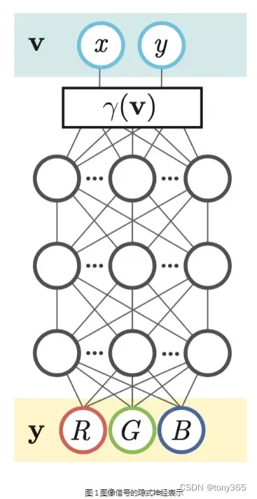
以图像信号的隐式神经表示举例:
对于图像v而言,对于每个图像平面内的像素点存在像素的坐标(x,y),同时存在每个像素的RGB值,使用一个神经网络学习坐标(x,y)和RGB值的关系,得到训练后的网络Φ。这里的Φ就是图像v的隐式神经表示。
[1]https://www.ipanqiao.com/entry/713
1. 了解SineLayer的初始化,还是没了解。。。
本文提出使用 sin 函数代替常规的relu等激活函数,来拟合更复杂的信息,sin 函数的使用增加了网络的结构复杂度,同时也提高了网络的表现能力。加入sin 函数后网络的参数初始化很重要,没有好的初始化会导致比较差的效果。
作者通过一系列证明推导出一个比较好的参数初始化方案。
初始化方案的关键思想是保持通过网络的激活的分布,这样初始化时的最终输出就不依赖于层数。
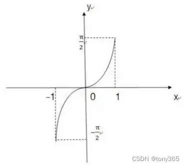
正弦函数y=sin x在[-π/2,π/2]上的反函数,叫做反正弦函数,记作arcsinx。
表示一个正弦值为x的角,该角的范围在[-π/2,π/2]区间内。
定义域[-1,1] ,值域[-π/2,π/2]。
(1) arcsinx是 (主值区)上的一个角(弧度数) 。
(2) 这个角(弧度数)的正弦值等于x,即sin(arcsinx)=x.
2. 均匀分布

3. Lemma 1.1
通过 arc sin函数和 均匀分布的知识,可以理解论文中的Lemma1.1 的推导过程。
![]()
其中 PDF 和 cdf 分别是
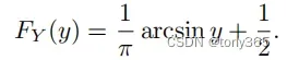
![]()
等等证明,没看太懂,直接看code吧
4. 一个简单实验, 拟合图像
4.1 网络模型代码如下,就是全连接网络,
但是激活函数是sine函数,另外就是SineLayer的初始化方法比较重要,论文中有大量证明。
class SineLayer(nn.Module):
    # See paper sec. 3.2, final paragraph, and supplement Sec. 1.5 for discussion of omega_0.

    # If is_first=True, omega_0 is a frequency factor which simply multiplies the activations before the
    # nonlinearity. Different signals may require different omega_0 in the first layer - this is a
    # hyperparameter.

    # If is_first=False, then the weights will be divided by omega_0 so as to keep the magnitude of
    # activations constant, but boost gradients to the weight matrix (see supplement Sec. 1.5)

    def __init__(self, in_features, out_features, bias=True,
                 is_first=False, omega_0=30):
        super().__init__()
        self.omega_0 = omega_0
        self.is_first = is_first

        self.in_features = in_features
        self.linear = nn.Linear(in_features, out_features, bias=bias)

        self.init_weights()

    def init_weights(self):
        with torch.no_grad():
            if self.is_first:
                self.linear.weight.uniform_(-1 / self.in_features,
                                             1 / self.in_features)
            else:
                self.linear.weight.uniform_(-np.sqrt(6 / self.in_features) / self.omega_0,
                                             np.sqrt(6 / self.in_features) / self.omega_0)

    def forward(self, input):
        return torch.sin(self.omega_0 * self.linear(input))

    def forward_with_intermediate(self, input):
        # For visualization of activation distributions
        intermediate = self.omega_0 * self.linear(input)
        return torch.sin(intermediate), intermediate


class Siren(nn.Module):
    def __init__(self, in_features, hidden_features, hidden_layers, out_features, outermost_linear=False,
                 first_omega_0=30, hidden_omega_0=30.):
        super().__init__()

        self.net = []
        self.net.append(SineLayer(in_features, hidden_features,
                                  is_first=True, omega_0=first_omega_0))

        for i in range(hidden_layers):
            self.net.append(SineLayer(hidden_features, hidden_features,
                                      is_first=False, omega_0=hidden_omega_0))

        if outermost_linear:
            final_linear = nn.Linear(hidden_features, out_features)

            with torch.no_grad():
                final_linear.weight.uniform_(-np.sqrt(6 / hidden_features) / hidden_omega_0,
                                              np.sqrt(6 / hidden_features) / hidden_omega_0)

            self.net.append(final_linear)
        else:
            self.net.append(SineLayer(hidden_features, out_features,
                                      is_first=False, omega_0=hidden_omega_0))

        self.net = nn.Sequential(*self.net)

    def forward(self, coords):
        coords = coords.clone().detach().requires_grad_(True) # allows to take derivative w.r.t. input
        output = self.net(coords)
        return output, coords

    def forward_with_activations(self, coords, retain_grad=False):
        '''Returns not only model output, but also intermediate activations.
        Only used for visualizing activations later!'''
        activations = OrderedDict()

        activation_count = 0
        x = coords.clone().detach().requires_grad_(True)
        activations['input'] = x
        for i, layer in enumerate(self.net):
            if isinstance(layer, SineLayer):
                x, intermed = layer.forward_with_intermediate(x)

                if retain_grad:
                    x.retain_grad()
                    intermed.retain_grad()

                activations['_'.join((str(layer.__class__), "%d" % activation_count))] = intermed
                activation_count += 1
            else:
                x = layer(x)

                if retain_grad:
                    x.retain_grad()

            activations['_'.join((str(layer.__class__), "%d" % activation_count))] = x
            activation_count += 1

        return activations
4.2 获取到图像
def laplace(y, x):
    grad = gradient(y, x)
    return divergence(grad, x)


def divergence(y, x):
    div = 0.
    for i in range(y.shape[-1]):
        div += torch.autograd.grad(y[..., i], x, torch.ones_like(y[..., i]), create_graph=True)[0][..., i:i + 1]
    return div


def gradient(y, x, grad_outputs=None):
    if grad_outputs is None:
        grad_outputs = torch.ones_like(y)
    grad = torch.autograd.grad(y, [x], grad_outputs=grad_outputs, create_graph=True)[0]
    return grad


def get_cameraman_tensor(sidelength):
    img = Image.fromarray(skimage.data.camera())
    transform = Compose([
        Resize(sidelength),
        ToTensor(),
        Normalize(torch.Tensor([0.5]), torch.Tensor([0.5]))
    ])
    img = transform(img)
    return img
import cv2
img0 = get_cameraman_tensor(128)
img0 = img0.cpu().permute(1,2,0).numpy().astype(np.float32)
#img1 = (img0 - img0.min()) / (img0.max() - img0.min())
plt.imshow(img0, 'gray')
plt.show()
4.3 训练
模型的输入是 像素坐标,输出是像素值
通过训练后即用网络参数来拟合一张图像
class ImageFitting(Dataset):
    def __init__(self, sidelength):
        super().__init__()
        img = get_cameraman_tensor(sidelength)
        self.pixels = img.permute(1, 2, 0).view(-1, 1)
        self.coords = get_mgrid(sidelength, 2)

    def __len__(self):
        return 1

    def __getitem__(self, idx):
        if idx > 0: raise IndexError

        return self.coords, self.pixels
训练方法比较常规
siz = 128
cameraman = ImageFitting(siz)
dataloader = DataLoader(cameraman, batch_size=1, pin_memory=True, num_workers=0)
img_siren = Siren(in_features=2, out_features=1, hidden_features=256,
hidden_layers=3, outermost_linear=True)
img_siren.cuda()
total_steps = 2501 # Since the whole image is our dataset, this just means 500 gradient descent steps.
steps_til_summary = 2500
optim = torch.optim.Adam(lr=1e-4, params=img_siren.parameters())
model_input, ground_truth = next(iter(dataloader))
model_input, ground_truth = model_input.cuda(), ground_truth.cuda()
for step in range(total_steps):
model_output, coords = img_siren(model_input)
loss = ((model_output - ground_truth) ** 2).mean()
if not step % steps_til_summary:
print("Step %d, Total loss %0.6f" % (step, loss))
img_grad = gradient(model_output, coords)
img_laplacian = laplace(model_output, coords)
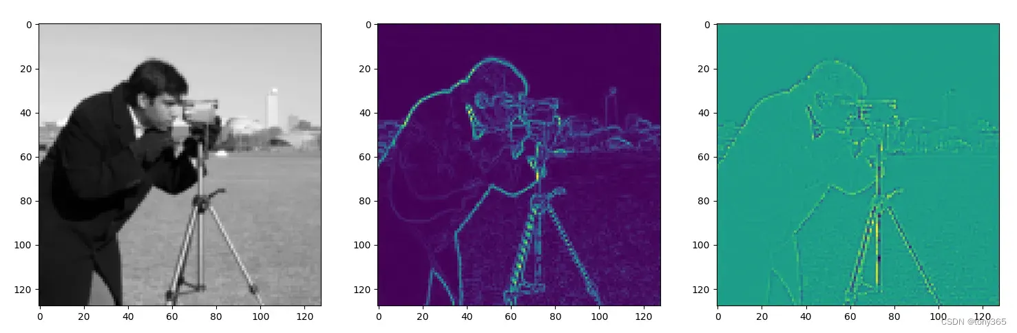
fig, axes = plt.subplots(1, 3, figsize=(18, 6))
axes[0].imshow(model_output.cpu().view(siz, siz).detach().numpy(), 'gray')
axes[1].imshow(img_grad.norm(dim=-1).cpu().view(siz, siz).detach().numpy(), 'gray')
axes[2].imshow(img_laplacian.cpu().view(siz, siz).detach().numpy(), 'gray')
plt.show()
optim.zero_grad()
loss.backward()
optim.step()
得到拟合的图像,一阶梯度图,二阶laplace 图像。
[1]https://github.com/vsitzmann/siren
文章出处登录后可见!