本文总结Numpy的用法,建议先学习python的container 基础。numpy可以理解列表或数组。
一个numpy数组是一个由不同数值组成的网格。网格中的数据都是同一种数据类型,可以通过非负整型数的元组来访问。维度的数量被称为数组的阶,数组的大小是一个由整型数构成的元组,可以描述数组不同维度上的大小。
1、创建一维数组
import numpy as np

a = np.array([1, 2, 3])  # Create a rank 1 array
print type(a)            # Prints "<type 'numpy.ndarray'>"
print a.shape            # Prints "(3,)"
print a[0], a[1], a[2]   # Prints "1 2 3"
a[0] = 5                 # Change an element of the array
print a                  # Prints "[5, 2, 3]"
2、创建二维数组
b = np.array([[1,2,3],[4,5,6]])   # Create a rank 2 array
print b                           # 显示一下矩阵b
print b.shape                     # Prints "(2, 3)"
print b[0, 0], b[0, 1], b[1, 0]   # Prints "1 2 4"
3、Numpy还提供了很多其他创建数组的方法
import numpy as np
#创建2行2列,值均为0的数组
a = np.zeros((2,2))  # Create an array of all zeros
print a              # Prints "[[ 0.  0.]
                     #          [ 0.  0.]]"
#创建1行2列,值均为1的数组
b = np.ones((1,2))   # Create an array of all ones
print b              # Prints "[[ 1.  1.]]"

#创建2行2列,值均为7的数组
c = np.full((2,2), 7) # Create a constant array
print c               # Prints "[[ 7.  7.]
                      #          [ 7.  7.]]"
#创建2行2列,斜线为1的数组
d = np.eye(2)        # Create a 2x2 identity matrix
print d              # Prints "[[ 1.  0.]
                     #          [ 0.  1.]]"
#创建2行2列的随机数组
e = np.random.random((2,2)) # Create an array filled with random values
print e # Might print "[[ 0.91940167 0.08143941]4、数组切片
和Python列表类似,numpy数组可以使用切片语法。因为数组可以是多维的,所以你必须为每个维度指定好切片。
import numpy as np

# 创建2维表,形状 3行4列
# [[ 1  2  3  4]
#  [ 5  6  7  8]
#  [ 9 10 11 12]]
a = np.array([[1,2,3,4], [5,6,7,8], [9,10,11,12]])

# 使用切片得到2行2列的子数组b
# :2指取0至1行,1:3指取1至2列
# [[2 3]
#  [6 7]]
b = a[:2, 1:3]

# 0指取0行,1指取1列
print a[0, 1]   # Prints "2"
b[0, 0] = 77    # b[0, 0] is the same piece of data as a[0, 1]

#当子数组更新,父数组也相应更新
print a[0, 1]   # Prints "77"
5、整型和切片语法
你可以同时使用整型和切片语法来访问数组。但是,这样做会产生一个比原数组低阶的新数组。需要注意的是,这里和MATLAB中的情况是不同的
# [[ 1  2  3  4]
#  [ 5  6  7  8]
#  [ 9 10 11 12]]
a = np.array([[1,2,3,4], [5,6,7,8], [9,10,11,12]])

# Two ways of accessing the data in the middle row of the array.
# Mixing integer indexing with slices yields an array of lower rank,
# while using only slices yields an array of the same rank as the
# original array:
row_r1 = a[1, :]    # Rank 1 view of the second row of a
row_r2 = a[1:2, :]  # Rank 2 view of the second row of a
print row_r1, row_r1.shape  # Prints "[5 6 7 8] (4,)"
print row_r2, row_r2.shape  # Prints "[[5 6 7 8]] (1, 4)"

# We can make the same distinction when accessing columns of an array:
col_r1 = a[:, 1]
col_r2 = a[:, 1:2]
print col_r1, col_r1.shape  # Prints "[ 2  6 10] (3,)"
print col_r2, col_r2.shape  # Prints "[[ 2]
                            #          [ 6]
# [10]] (3, 1)"6、整型数组访问
当我们使用切片语法访问数组时,得到的总是原数组的一个子集。整型数组访问允许我们利用其它数组的数据构建一个新的数组:
import numpy as np

a = np.array([[1,2], [3, 4], [5, 6]])

# An example of integer array indexing.
# The returned array will have shape (3,) and
# [0, 1, 2]指第0,1,2行,[0, 1, 0]指第0,1,0列
print a[[0, 1, 2], [0, 1, 0]]  # Prints "[1 4 5]"

# The above example of integer array indexing is equivalent to this:
print np.array([a[0, 0], a[1, 1], a[2, 0]])  # Prints "[1 4 5]"

# When using integer array indexing, you can reuse the same
# element from the source array:
a[[0, 0], [1, 1]] 相当于 a[0, 1]
print a[[0, 0], [1, 1]]  # Prints "[2 2]"

# Equivalent to the previous integer array indexing example
print np.array([a[0, 1], a[0, 1]])  # Prints "[2 2]"
7、选择或者更改元素
整型数组访问语法还有个有用的技巧,可以用来选择或者更改矩阵中每行中的一个元素:
import numpy as np

# Create a new array from which we will select elements
a = np.array([[1,2,3], [4,5,6], [7,8,9], [10, 11, 12]])

print a  # prints "array([[ 1,  2,  3],
         #                [ 4,  5,  6],
         #                [ 7,  8,  9],
         #                [10, 11, 12]])"

# Create an array of indices
b = np.array([0, 2, 0, 1])

# Select one element from each row of a using the indices in b
#np.arange(4)指按顺序从0至3数,相当于数组[0,1,2,3],即是指定了第0-3行
#b  [0, 2, 0, 1] 是取a数组的第0,2,0,1列
print a[np.arange(4), b]  # Prints "[ 1  6  7 11]"

# Mutate one element from each row of a using the indices in b
a[np.arange(4), b] += 10
#以上指定的元素,均加10
print a  # prints "array([[11,  2,  3],
         #                [ 4,  5, 16],
         #                [17,  8,  9],
# [10, 21, 12]])8、布尔型数组访问
布尔型数组访问可以让你选择数组中任意元素。通常,这种访问方式用于选取数组中满足某些条件的元素,举例如下:
import numpy as np

a = np.array([[1,2], [3, 4], [5, 6]])

bool_idx = (a > 2)  # Find the elements of a that are bigger than 2;
                    # this returns a numpy array of Booleans of the same
                    # shape as a, where each slot of bool_idx tells
                    # whether that element of a is > 2.

print bool_idx      # Prints "[[False False]
                    #          [ True  True]
                    #          [ True  True]]"

# We use boolean array indexing to construct a rank 1 array
# consisting of the elements of a corresponding to the True values
# of bool_idx
print a[bool_idx]  # Prints "[3 4 5 6]"

# We can do all of the above in a single concise statement:
print a[a > 2]     # Prints "[3 4 5 6]"
有很多数组访问的细节我们没有详细说明,可以查看文档。
9、数据类型
每个Numpy数组都是数据类型相同的元素组成的网格。Numpy提供了很多的数据类型用于创建数组。当你创建数组的时候,Numpy会尝试猜测数组的数据类型,你也可以通过参数直接指定数据类型,例子如下:
import numpy as np

x = np.array([1, 2])  # Let numpy choose the datatype
print x.dtype         # Prints "int64"

x = np.array([1.0, 2.0])  # Let numpy choose the datatype
print x.dtype             # Prints "float64"

x = np.array([1, 2], dtype=np.int64)  # Force a particular datatype
print x.dtype                         # Prints "int64"
更多细节查看文档。
10、数组计算
基本数学计算函数会对数组中元素逐个进行计算,既可以利用操作符重载,也可以使用函数方式:
import numpy as np

x = np.array([[1,2],[3,4]], dtype=np.float64)
y = np.array([[5,6],[7,8]], dtype=np.float64)

# Elementwise sum; both produce the array
# [[ 6.0  8.0]
#  [10.0 12.0]]
print x + y
print np.add(x, y)

# Elementwise difference; both produce the array
# [[-4.0 -4.0]
#  [-4.0 -4.0]]
print x - y
print np.subtract(x, y)

# Elementwise product; both produce the array
# [[ 5.0 12.0]
#  [21.0 32.0]]
print x * y
print np.multiply(x, y)

# Elementwise division; both produce the array
# [[ 0.2         0.33333333]
#  [ 0.42857143  0.5       ]]
print x / y
print np.divide(x, y)

# Elementwise square root; produces the array
# [[ 1.          1.41421356]
#  [ 1.73205081  2.        ]]
print np.sqrt(x)
11、dot矩阵乘法
和MATLAB不同,*是元素逐个相乘,而不是矩阵乘法。在Numpy中使用dot来进行矩阵乘法,计算矩阵乘法,请将第一个矩阵行元素(或数字)乘以第二个矩阵列元素,然后计算其总和:
import numpy as np

x = np.array([[1,2],[3,4]])
y = np.array([[5,6],[7,8]])

v = np.array([9,10])
w = np.array([11, 12])

# Inner product of vectors; both produce 219
print v.dot(w)
print np.dot(v, w)

# Matrix / vector product; both produce the rank 1 array [29 67]
print x.dot(v)
print np.dot(x, v)

# Matrix / matrix product; both produce the rank 2 array
# [[19 22]
#  [43 50]]
#计算过程:1*5+2*7=19,1*6+2*8=22,其他依此类计算
print x.dot(y)
print np.dot(x, y)
12、sum函数
Numpy提供了很多计算数组的函数,其中最常用的一个是sum:
import numpy as np

x = np.array([[1,2],[3,4]])

print np.sum(x)  # Compute sum of all elements; prints "10"
#axis=0 列相加;axis=1 行相加。
print np.sum(x, axis=0)  # Compute sum of each column; prints "[4 6]"
print np.sum(x, axis=1)  # Compute sum of each row; prints "[3 7]"
想要了解更多函数,可以查看文档。
13、T转置矩阵
除了计算,我们还常常改变数组或者操作其中的元素。其中将矩阵转置是常用的一个,在Numpy中,使用T来转置矩阵:
import numpy as np

x = np.array([[1,2], [3,4]])
print x    # Prints "[[1 2]
           #          [3 4]]"
print x.T  # Prints "[[1 3]
           #          [2 4]]"

# Note that taking the transpose of a rank 1 array does nothing:
v = np.array([1,2,3])
print v    # Prints "[1 2 3]"
print v.T  # Prints "[1 2 3]"
Numpy还提供了更多操作数组的方法,请查看文档。
14、广播Broadcasting
广播是一种强有力的机制,它让Numpy可以让不同大小的矩阵在一起进行数学计算。我们常常会有一个小的矩阵和一个大的矩阵,然后我们会需要用小的矩阵对大的矩阵做一些计算。
举个例子,如果我们想要把一个向量加到矩阵的每一行,我们可以这样做:
import numpy as np

# We will add the vector v to each row of the matrix x,
# storing the result in the matrix y
x = np.array([[1,2,3], [4,5,6], [7,8,9], [10, 11, 12]])
v = np.array([1, 0, 1])
y = np.empty_like(x)   # Create an empty matrix with the same shape as x

# Add the vector v to each row of the matrix x with an explicit loop
for i in range(4):
    y[i, :] = x[i, :] + v

# Now y is the following
# [[ 2  2  4]
#  [ 5  5  7]
#  [ 8  8 10]
#  [11 11 13]]
print y
这样是行得通的,但是当x矩阵非常大,利用循环来计算就会变得很慢很慢。我们可以换一种思路:
import numpy as np

# We will add the vector v to each row of the matrix x,
# storing the result in the matrix y
x = np.array([[1,2,3], [4,5,6], [7,8,9], [10, 11, 12]])
v = np.array([1, 0, 1])
vv = np.tile(v, (4, 1))  # Stack 4 copies of v on top of each other
print vv                 # Prints "[[1 0 1]
                         #          [1 0 1]
                         #          [1 0 1]
                         #          [1 0 1]]"
y = x + vv  # Add x and vv elementwise
print y  # Prints "[[ 2  2  4
         #          [ 5  5  7]
         #          [ 8  8 10]
         #          [11 11 13]]"
Numpy广播机制可以让我们不用创建vv,就能直接运算,看看下面例子:
import numpy as np

# We will add the vector v to each row of the matrix x,
# storing the result in the matrix y
x = np.array([[1,2,3], [4,5,6], [7,8,9], [10, 11, 12]])
v = np.array([1, 0, 1])
y = x + v  # Add v to each row of x using broadcasting
print y  # Prints "[[ 2  2  4]
         #          [ 5  5  7]
         #          [ 8  8 10]
         #          [11 11 13]]"
对两个数组使用广播机制要遵守下列规则:
如果数组的秩不同,使用1来将秩较小的数组进行扩展,直到两个数组的尺寸的长度都一样。
如果两个数组在某个维度上的长度是一样的,或者其中一个数组在该维度上长度为1,那么我们就说这两个数组在该维度上是相容的。
如果两个数组在所有维度上都是相容的,他们就能使用广播。
如果两个输入数组的尺寸不同,那么注意其中较大的那个尺寸。因为广播之后,两个数组的尺寸将和那个较大的尺寸一样。
在任何一个维度上,如果一个数组的长度为1,另一个数组长度大于1,那么在该维度上,就好像是对第一个数组进行了复制。
如果上述解释看不明白,可以读一读文档和这个解释。译者注:强烈推荐阅读文档中的例子。
支持广播机制的函数是全局函数。哪些是全局函数可以在文档中查找。
下面是一些广播机制的使用:
import numpy as np

# Compute outer product of vectors
v = np.array([1,2,3])  # v has shape (3,)
w = np.array([4,5])    # w has shape (2,)
# To compute an outer product, we first reshape v to be a column
# vector of shape (3, 1); we can then broadcast it against w to yield
# an output of shape (3, 2), which is the outer product of v and w:
# [[ 4  5]
#  [ 8 10]
#  [12 15]]
print np.reshape(v, (3, 1)) * w

# Add a vector to each row of a matrix
x = np.array([[1,2,3], [4,5,6]])
# x has shape (2, 3) and v has shape (3,) so they broadcast to (2, 3),
# giving the following matrix:
# [[2 4 6]
#  [5 7 9]]
print x + v

# Add a vector to each column of a matrix
# x has shape (2, 3) and w has shape (2,).
# If we transpose x then it has shape (3, 2) and can be broadcast
# against w to yield a result of shape (3, 2); transposing this result
# yields the final result of shape (2, 3) which is the matrix x with
# the vector w added to each column. Gives the following matrix:
# [[ 5  6  7]
#  [ 9 10 11]]
print (x.T + w).T

# Another solution is to reshape w to be a row vector of shape (2, 1);
# we can then broadcast it directly against x to produce the same
# output.
print x + np.reshape(w, (2, 1))

# Multiply a matrix by a constant:
# x has shape (2, 3). Numpy treats scalars as arrays of shape ();
# these can be broadcast together to shape (2, 3), producing the
# following array:
# [[ 2  4  6]
#  [ 8 10 12]]
print x * 2
广播机制能够让你的代码更简洁更迅速,能够用的时候请尽量使用!
15、SciPy
Numpy提供了高性能的多维数组,以及计算和操作数组的基本工具。SciPy基于Numpy,提供了大量的计算和操作数组的函数,这些函数对于不同类型的科学和工程计算非常有用。
熟悉SciPy的最好方法就是阅读文档。我们会强调对于本课程有用的部分。
- 图像操作
SciPy提供了一些操作图像的基本函数。比如,它提供了将图像从硬盘读入到数组的函数,也提供了将数组中数据写入的硬盘成为图像的函数。下面是一个简单的例子:
from scipy.misc import imread, imsave, imresize

# Read an JPEG image into a numpy array
img = imread('assets/cat.jpg')
print img.dtype, img.shape  # Prints "uint8 (400, 248, 3)"

# We can tint the image by scaling each of the color channels
# by a different scalar constant. The image has shape (400, 248, 3);
# we multiply it by the array [1, 0.95, 0.9] of shape (3,);
# numpy broadcasting means that this leaves the red channel unchanged,
# and multiplies the green and blue channels by 0.95 and 0.9
# respectively.
img_tinted = img * [1, 0.95, 0.9]

# Resize the tinted image to be 300 by 300 pixels.
img_tinted = imresize(img_tinted, (300, 300))

# Write the tinted image back to disk
imsave('assets/cat_tinted.jpg', img_tinted)
2、点之间的距离
SciPy定义了一些有用的函数,可以计算集合中点之间的距离。
函数scipy.spatial.distance.pdist能够计算集合中所有两点之间的距离:
import numpy as np
from scipy.spatial.distance import pdist, squareform

# Create the following array where each row is a point in 2D space:
# [[0 1]
#  [1 0]
#  [2 0]]
x = np.array([[0, 1], [1, 0], [2, 0]])
print x

# Compute the Euclidean distance between all rows of x.
# d[i, j] is the Euclidean distance between x[i, :] and x[j, :],
# and d is the following array:
# [[ 0.          1.41421356  2.23606798]
#  [ 1.41421356  0.          1.        ]
#  [ 2.23606798  1.          0.        ]]
d = squareform(pdist(x, 'euclidean'))
print d
具体细节请阅读文档。
函数scipy.spatial.distance.cdist可以计算不同集合中点的距离,具体请查看文档。
16、Matplotlib
Matplotlib是一个作图库。这里简要介绍matplotlib.pyplot模块,功能和MATLAB的作图功能类似。
绘图。matplotlib库中最重要的函数是Plot。该函数允许你做出2D图形,如下:
import numpy as np
import matplotlib.pyplot as plt

# Compute the x and y coordinates for points on a sine curve
x = np.arange(0, 3 * np.pi, 0.1)
y = np.sin(x)

# Plot the points using matplotlib
plt.plot(x, y)
plt.show()  # You must call plt.show() to make graphics appear.
只需要少量工作,就可以一次画不同的线,加上标签,坐标轴标志等。
import numpy as np
import matplotlib.pyplot as plt

# Compute the x and y coordinates for points on sine and cosine curves
x = np.arange(0, 3 * np.pi, 0.1)
y_sin = np.sin(x)
y_cos = np.cos(x)

# Plot the points using matplotlib
plt.plot(x, y_sin)
plt.plot(x, y_cos)
plt.xlabel('x axis label')
plt.ylabel('y axis label')
plt.title('Sine and Cosine')
plt.legend(['Sine', 'Cosine'])
plt.show()
绘制多个图像,可以使用subplot函数来在一幅图中画不同的东西:
import numpy as np
import matplotlib.pyplot as plt

# Compute the x and y coordinates for points on sine and cosine curves
x = np.arange(0, 3 * np.pi, 0.1)
y_sin = np.sin(x)
y_cos = np.cos(x)

# Set up a subplot grid that has height 2 and width 1,
# and set the first such subplot as active.
plt.subplot(2, 1, 1)

# Make the first plot
plt.plot(x, y_sin)
plt.title('Sine')

# Set the second subplot as active, and make the second plot.
plt.subplot(2, 1, 2)
plt.plot(x, y_cos)
plt.title('Cosine')

# Show the figure.
plt.show()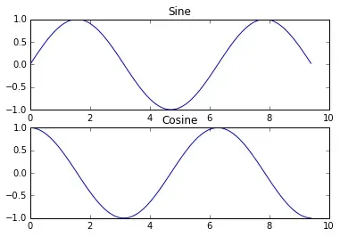
你可以使用imshow函数来显示图像,如下所示:
import numpy as np
from scipy.misc import imread, imresize
import matplotlib.pyplot as plt

img = imread('assets/cat.jpg')
img_tinted = img * [1, 0.95, 0.9]

# Show the original image
plt.subplot(1, 2, 1)
plt.imshow(img)

# Show the tinted image
plt.subplot(1, 2, 2)

# A slight gotcha with imshow is that it might give strange results
# if presented with data that is not uint8. To work around this, we
# explicitly cast the image to uint8 before displaying it.
plt.imshow(np.uint8(img_tinted))
plt.show()
文章出处登录后可见!