前言

大家好，我是阿光。

本专栏整理了《图神经网络代码实战》，内包含了不同图神经网络的相关代码实现（PyG以及自实现），理论与实践相结合，如GCN、GAT、GraphSAGE等经典图网络，每一个代码实例都附带有完整的代码。

正在更新中~ ✨

在这里插入图片描述

🚨 我的项目环境：

平台：Windows10
语言环境：python3.7
编译器：PyCharm
PyTorch版本：1.11.0
PyG版本：2.1.0

💥 项目专栏：【图神经网络代码实战目录】

本文我们将使用PyTorch来简易实现一个GAT（图注意力网络），不使用PyG库，让新手可以理解如何PyTorch来搭建一个简易的图网络实例demo。

一、导入相关库

本项目是采用自己实现的GAT，并没有使用 PyG 库，原因是为了帮助新手朋友们能够对GAT的原理有个更深刻的理解，如果熟悉之后可以尝试使用PyG库直接调用 GATConv 这个图层即可。

import numpy as np
import torch
import torch.nn as nn
import torch.nn.functional as F
from scipy.sparse import coo_matrix
from torch_geometric.datasets import Planetoid

二、加载Cora数据集

本文使用的数据集是比较经典的Cora数据集，它是一个根据科学论文之间相互引用关系而构建的Graph数据集合，论文分为7类，共2708篇。

Genetic_Algorithms
Neural_Networks
Probabilistic_Methods
Reinforcement_Learning
Rule_Learning
Theory

这个数据集是一个用于图节点分类的任务，数据集中只有一张图，这张图中含有2708个节点，10556条边，每个节点的特征维度为1433。

# 1.加载Cora数据集
dataset = Planetoid(root='./data/Cora', name='Cora')

三、定义GAT网络

3.1 定义GAT层

这里我们就不重点介绍GCN网络了，相信大家能够掌握基本原理，本文我们使用的是PyTorch定义网络层。

在这里插入图片描述

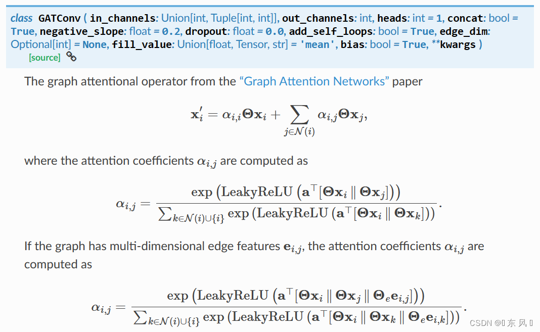
对于GATConv的常用参数：

in_channels：每个样本的输入维度，就是每个节点的特征维度
out_channels：经过注意力机制后映射成的新的维度，就是经过GAT后每个节点的维度长度
add_self_loops：为图添加自环，是否考虑自身节点的信息
bias：训练一个偏置b

我们在实现时也是考虑这几个常见参数

对于GAT的传播公式为：

Pytorch实现GAT(基于PyTorch实现)

上式子的意思就是对自己和邻居的特征进行按照权重聚合，其中的 Pytorch实现GAT(基于PyTorch实现) 代表注意力分数，代表可学习参数，代表邻居节点的特征向量。

其中注意力分数的计算方式如下：

Pytorch实现GAT(基于PyTorch实现)

所以我们的任务无非就是获取这几个变量，然后进行传播计算即可

3.1.1 将节点信息进行空间映射

在注意力公式中，它是首先对邻居节点先进行空间上的映射，实现代码如下：

# 1.计算wh，进行节点空间映射
wh = torch.mm(x, self.weight_w)

3.1.2 注意力分数

第二步就是计算注意力分数，注意一点这个分数并没有被激活，实现的部分就是 LeakyReLU 括号内的部分。

# 2.计算注意力分数
e = torch.mm(wh, self.weight_a[: self.out_channels]) + torch.matmul(wh, self.weight_a[self.out_channels:]).T

3.1.3 获取邻接矩阵

由于我们使用的是内置数据集 Cora，他给出的数据集并没有给出对应的邻接矩阵，所以我们需要手动实现获取该图对应的邻接矩阵。

# 4.获取邻接矩阵
if self.adj == None:
    self.adj = to_dense_adj(edge_index).squeeze()
    
    # 5.添加自环，考虑自身加权
    if self.add_self_loops:
        self.adj += torch.eye(x.shape[0])

3.1.4 获得注意力分数矩阵

在上述GAT的传播公式中我们可以看到，每次加权的节点信息为自身和其邻居节点，所以为了实现非邻居节点不参与加权，我们需要对注意力分数矩阵非邻居节点的位置将其置为一个很小的值，这样在矩阵乘法时就不会发挥什么作用。

# 6.获得注意力分数矩阵
attention = torch.where(self.adj > 0, e, -1e9 * torch.ones_like(e))

该代码的意思就是如果邻接矩阵中位置大于0，也就是该条边存在，那么注意力矩阵对应的位置分数不变，否则将其置为 -1e9 这个很小的数。

3.1.5 加权融合特征

这个部分就是将获得的注意力分数进行归一化，然后将这个矩阵和映射后的特征矩阵进行相乘，实现聚合操作，最终在结果上面添加偏置信息。

# 7.归一化注意力分数
attention = F.softmax(attention, dim=1)

# 8.加权融合特征
output = torch.mm(attention, wh)

# 9.添加偏置
if self.bias != None:
    return output + self.bias.flatten()
else:
    return output

3.1.6 GATConv层

接下来就可以定义GATConv层了，该层实现了2个函数，分别是 init_parameters() 、forward()

init_parameters()：初始化可学习参数
forward()：这个函数定义模型的传播过程，也就是上面公式的，如果设置了偏置在加上偏置返回即可

# 2.定义GATConv层
class GATConv(nn.Module):
    def __init__(self, in_channels, out_channels, heads=1, add_self_loops=True, bias=True):
        super(GATConv, self).__init__()
        self.in_channels = in_channels # 输入图节点的特征数
        self.out_channels = out_channels # 输出图节点的特征数
        self.adj = None
        self.add_self_loops = add_self_loops
        
        
        # 定义参数 θ
        self.weight_w = nn.Parameter(torch.FloatTensor(in_channels, out_channels))
        self.weight_a = nn.Parameter(torch.FloatTensor(out_channels * 2, 1))
        
        if bias:
            self.bias = nn.Parameter(torch.FloatTensor(out_channels, 1))
        else:
            self.register_parameter('bias', None)
        
        self.leakyrelu = nn.LeakyReLU()
        self.init_parameters()
    
    # 初始化可学习参数
    def init_parameters(self):
        nn.init.xavier_uniform_(self.weight_w)
        nn.init.xavier_uniform_(self.weight_a)
        
        if self.bias != None:
            nn.init.zeros_(self.bias)
        
    def forward(self, x, edge_index):
        # 1.计算wh，进行节点空间映射
        wh = torch.mm(x, self.weight_w)
                                  
        # 2.计算注意力分数
        e = torch.mm(wh, self.weight_a[: self.out_channels]) + torch.matmul(wh, self.weight_a[self.out_channels:]).T

        # 3.激活
        e = self.leakyrelu(e)
        
        # 4.获取邻接矩阵
        if self.adj == None:
            self.adj = to_dense_adj(edge_index).squeeze()
            
            # 5.添加自环，考虑自身加权
            if self.add_self_loops:
                self.adj += torch.eye(x.shape[0])
        
        # 6.获得注意力分数矩阵
        attention = torch.where(self.adj > 0, e, -1e9 * torch.ones_like(e))
        
        # 7.归一化注意力分数
        attention = F.softmax(attention, dim=1)
        
        # 8.加权融合特征
        output = torch.mm(attention, wh)
        
        # 9.添加偏置
        if self.bias != None:
            return output + self.bias.flatten()
        else:
            return output

对于我们实现这个网络的实现效率上来讲比PyG框架内置的 GCNConv 层稍差一点，因为我们是按照公式来一步一步利用矩阵计算得到，没有对矩阵计算以及算法进行优化，不然初学者可能看不太懂，不利于理解GCN公式的传播过程，有能力的小伙伴可以看下官方源码学习一下。

3.2 定义GAT网络

上面我们已经实现好了 GATConv 的网络层，之后就可以调用这个层来搭建 GAT 网络。

# 3.定义GAT网络
class GAT(nn.Module):
    def __init__(self, num_node_features, num_classes):
        super(GAT, self).__init__()
        self.conv1 = GATConv(in_channels=num_node_features,
                                    out_channels=16,
                                    heads=2)
        self.conv2 = GATConv(in_channels=16,
                                    out_channels=num_classes,
                                    heads=1)
        
    def forward(self, data):
        x, edge_index = data.x, data.edge_index
        
        x = self.conv1(x, edge_index)
        x = F.relu(x)
        x = F.dropout(x, training=self.training)
        x = self.conv2(x, edge_index)
        
        return F.log_softmax(x, dim=1)

上面网络我们定义了两个GATConv层，第一层的参数的输入维度就是初始每个节点的特征维度，输出维度是16。

第二个层的输入维度为16，输出维度为分类个数，因为我们需要对每个节点进行分类，最终加上softmax操作。

四、定义模型

下面就是定义了一些模型需要的参数，像学习率、迭代次数这些超参数，然后是模型的定义以及优化器及损失函数的定义，和pytorch定义网络是一样的。

device = torch.device('cuda' if torch.cuda.is_available() else 'cpu') # 设备
epochs = 10 # 学习轮数
lr = 0.003 # 学习率
num_node_features = dataset.num_node_features # 每个节点的特征数
num_classes = dataset.num_classes # 每个节点的类别数
data = dataset[0].to(device) # Cora的一张图

# 3.定义模型
model = GAT(num_node_features, num_classes).to(device)
optimizer = torch.optim.Adam(model.parameters(), lr=lr) # 优化器
loss_function = nn.NLLLoss() # 损失函数

五、模型训练

模型训练部分也是和pytorch定义网络一样，因为都是需要经过前向传播、反向传播这些过程，对于损失、精度这些指标可以自己添加。

# 训练模式
model.train()

for epoch in range(epochs):
    optimizer.zero_grad()
    pred = model(data)
    
    loss = loss_function(pred[data.train_mask], data.y[data.train_mask]) # 损失
    correct_count_train = pred.argmax(axis=1)[data.train_mask].eq(data.y[data.train_mask]).sum().item() # epoch正确分类数目
    acc_train = correct_count_train / data.train_mask.sum().item() # epoch训练精度
    
    loss.backward()
    optimizer.step()
    
    if epoch % 20 == 0:
        print("【EPOCH: 】%s" % str(epoch + 1))
        print('训练损失为：{:.4f}'.format(loss.item()), '训练精度为：{:.4f}'.format(acc_train))

print('【Finished Training！】')

六、模型验证

下面就是模型验证阶段，在训练时我们是只使用了训练集，测试的时候我们使用的是测试集，注意这和传统网络测试不太一样，在图像分类一些经典任务中，我们是把数据集分成了两份，分别是训练集、测试集，但是在Cora这个数据集中并没有这样，它区分训练集还是测试集使用的是掩码机制，就是定义了一个和节点长度相同纬度的数组，该数组的每个位置为True或者False，标记着是否使用该节点的数据进行训练。

# 模型验证
model.eval()
pred = model(data)

# 训练集（使用了掩码）
correct_count_train = pred.argmax(axis=1)[data.train_mask].eq(data.y[data.train_mask]).sum().item()
acc_train = correct_count_train / data.train_mask.sum().item()
loss_train = loss_function(pred[data.train_mask], data.y[data.train_mask]).item()

# 测试集
correct_count_test = pred.argmax(axis=1)[data.test_mask].eq(data.y[data.test_mask]).sum().item()
acc_test = correct_count_test / data.test_mask.sum().item()
loss_test = loss_function(pred[data.test_mask], data.y[data.test_mask]).item()

print('Train Accuracy: {:.4f}'.format(acc_train), 'Train Loss: {:.4f}'.format(loss_train))
print('Test  Accuracy: {:.4f}'.format(acc_test), 'Test  Loss: {:.4f}'.format(loss_test))

七、结果

【EPOCH: 】1
训练损失为：1.9481 训练精度为：0.0714
【EPOCH: 】21
训练损失为：1.8783 训练精度为：0.3571
【EPOCH: 】41
训练损失为：1.7687 训练精度为：0.6071
【EPOCH: 】61
训练损失为：1.6368 训练精度为：0.7143
【EPOCH: 】81
训练损失为：1.5093 训练精度为：0.7500
【EPOCH: 】101
训练损失为：1.3747 训练精度为：0.8214
【EPOCH: 】121
训练损失为：1.2433 训练精度为：0.8500
【EPOCH: 】141
训练损失为：1.1180 训练精度为：0.8714
【EPOCH: 】161
训练损失为：1.0113 训练精度为：0.9000
【EPOCH: 】181
训练损失为：0.9571 训练精度为：0.8714
【Finished Training！】

>>>Train Accuracy: 0.9857 Train Loss: 0.8360
>>>Test  Accuracy: 0.7460 Test  Loss: 1.2454

训练集	测试集
Accuracy	0.9857	0.7460
Loss	0.8360	1.2454

完整代码

import numpy as np
import torch
import torch.nn as nn
import torch.nn.functional as F
from scipy.sparse import coo_matrix
from torch_geometric.datasets import Planetoid

# 1.加载Cora数据集
dataset = Planetoid(root='./data/Cora', name='Cora')

# 2.定义GATConv层
class GATConv(nn.Module):
    def __init__(self, in_channels, out_channels, heads=1, add_self_loops=True, bias=True):
        super(GATConv, self).__init__()
        self.in_channels = in_channels # 输入图节点的特征数
        self.out_channels = out_channels # 输出图节点的特征数
        self.adj = None
        self.add_self_loops = add_self_loops
        
        
        # 定义参数 θ
        self.weight_w = nn.Parameter(torch.FloatTensor(in_channels, out_channels))
        self.weight_a = nn.Parameter(torch.FloatTensor(out_channels * 2, 1))
        
        if bias:
            self.bias = nn.Parameter(torch.FloatTensor(out_channels, 1))
        else:
            self.register_parameter('bias', None)
        
        self.leakyrelu = nn.LeakyReLU()
        self.init_parameters()
    
    # 初始化可学习参数
    def init_parameters(self):
        nn.init.xavier_uniform_(self.weight_w)
        nn.init.xavier_uniform_(self.weight_a)
        
        if self.bias != None:
            nn.init.zeros_(self.bias)
        
    def forward(self, x, edge_index):
        # 1.计算wh，进行节点空间映射
        wh = torch.mm(x, self.weight_w)
                                  
        # 2.计算注意力分数
        e = torch.mm(wh, self.weight_a[: self.out_channels]) + torch.matmul(wh, self.weight_a[self.out_channels:]).T

        # 3.激活
        e = self.leakyrelu(e)
        
        # 4.获取邻接矩阵
        if self.adj == None:
            self.adj = to_dense_adj(edge_index).squeeze()
            
            # 5.添加自环，考虑自身加权
            if self.add_self_loops:
                self.adj += torch.eye(x.shape[0])
        
        # 6.获得注意力分数矩阵
        attention = torch.where(self.adj > 0, e, -1e9 * torch.ones_like(e))
        
        # 7.归一化注意力分数
        attention = F.softmax(attention, dim=1)
        
        # 8.加权融合特征
        output = torch.mm(attention, wh)
        
        # 9.添加偏置
        if self.bias != None:
            return output + self.bias.flatten()
        else:
            return output                                   

# 3.定义GAT网络
class GAT(nn.Module):
    def __init__(self, num_node_features, num_classes):
        super(GAT, self).__init__()
        self.conv1 = GATConv(in_channels=num_node_features,
                                    out_channels=16,
                                    heads=2)
        self.conv2 = GATConv(in_channels=16,
                                    out_channels=num_classes,
                                    heads=1)
        
    def forward(self, data):
        x, edge_index = data.x, data.edge_index
        
        x = self.conv1(x, edge_index)
        x = F.relu(x)
        x = F.dropout(x, training=self.training)
        x = self.conv2(x, edge_index)
        
        return F.log_softmax(x, dim=1)

device = torch.device('cuda' if torch.cuda.is_available() else 'cpu') # 设备
epochs = 200 # 学习轮数
lr = 0.0003 # 学习率
num_node_features = dataset.num_node_features # 每个节点的特征数
num_classes = dataset.num_classes # 每个节点的类别数
data = dataset[0].to(device) # Cora的一张图

# 4.定义模型
model = GCN(num_node_features, num_classes).to(device)
optimizer = torch.optim.Adam(model.parameters(), lr=lr) # 优化器
loss_function = nn.NLLLoss() # 损失函数

# 训练模式
model.train()

for epoch in range(epochs):
    optimizer.zero_grad()
    pred = model(data)
    
    loss = loss_function(pred[data.train_mask], data.y[data.train_mask]) # 损失
    correct_count_train = pred.argmax(axis=1)[data.train_mask].eq(data.y[data.train_mask]).sum().item() # epoch正确分类数目
    acc_train = correct_count_train / data.train_mask.sum().item() # epoch训练精度
    
    loss.backward()
    optimizer.step()
    
    if epoch % 20 == 0:
        print("【EPOCH: 】%s" % str(epoch + 1))
        print('训练损失为：{:.4f}'.format(loss.item()), '训练精度为：{:.4f}'.format(acc_train))

print('【Finished Training！】')

# 模型验证
model.eval()
pred = model(data)

# 训练集（使用了掩码）
correct_count_train = pred.argmax(axis=1)[data.train_mask].eq(data.y[data.train_mask]).sum().item()
acc_train = correct_count_train / data.train_mask.sum().item()
loss_train = loss_function(pred[data.train_mask], data.y[data.train_mask]).item()

# 测试集
correct_count_test = pred.argmax(axis=1)[data.test_mask].eq(data.y[data.test_mask]).sum().item()
acc_test = correct_count_test / data.test_mask.sum().item()
loss_test = loss_function(pred[data.test_mask], data.y[data.test_mask]).item()

print('Train Accuracy: {:.4f}'.format(acc_train), 'Train Loss: {:.4f}'.format(loss_train))
print('Test  Accuracy: {:.4f}'.format(acc_test), 'Test  Loss: {:.4f}'.format(loss_test))

文章出处登录后可见！

已经登录？立即刷新

Pytorch实现GAT(基于PyTorch实现)

文章目录

前言

一、导入相关库

二、加载Cora数据集

三、定义GAT网络

3.1 定义GAT层

3.1.1 将节点信息进行空间映射

3.1.2 注意力分数

3.1.3 获取邻接矩阵

3.1.4 获得注意力分数矩阵

3.1.5 加权融合特征

3.1.6 GATConv层

3.2 定义GAT网络

四、定义模型

五、模型训练

六、模型验证

七、结果

完整代码

相关推荐