高斯过程回归(Gaussian Processes Regression, GPR)简介
一、高斯过程简介
高斯过程是一种常用的监督学习方法,可以用于解决回归和分类问题。
高斯过程模型的优点有:
- 预测对观察结果进行了插值
- 预测的结果是概率形式的
- 通用性:可以指定不同的核函数(kernels)形式
高斯过程模型的确定包括:
- 它们不是稀疏的,即它们使用整个样本/特征信息来执行预测
- 高维空间模型会失效,高维也就是指特征的数量超过几十个
值得注意的是,高斯过程模型的优势主要体现在处理非线性和小数据问题上。
参考资料:https://scikit-learn.org/stable/modules/gaussian_process.html
二、高斯分布
1. 一元高斯分布
若一个随机变量服从均值为
,方差为
的高斯分布,则将其写作
,其概率密度函数形式为:
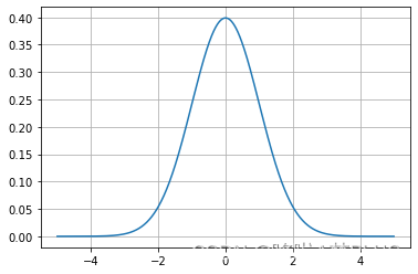
对于均值为0,方差为1的高斯分布可以画出其函数图像:
import matplotlib.pyplot as plt
import numpy as np

x = np.linspace(-5, 5, 10000)
y = 1.0/np.sqrt(2.0*np.pi)*np.exp(-1.0*np.power(x, 2)/2.0)
plt.plot(x, y)
plt.grid()
2. 多元高斯分布
对于任意维度的随机变量,其高斯分布可以写作
,其中
为协方差矩阵,其概率密度函数形式为:
其中协方差矩阵的形式为:
其中
其中c代表样本总数,协方差矩阵反映了不同变量之间的相关性大小,如果各个变量之间不相关,那么该矩阵为单位阵。关于多元高斯分布的一个重要性质就是:多元高斯分布的条件分布同样符合高斯分布。
三、高斯过程回归
顾名思义,高斯过程回归就是通过高斯过程来求解回归问题,回归是指通过适当的建模来拟合一组自变量和因变量
之间的函数关系,建模的方式有很多种,最常用的有线性回归,多项式回归等,高斯过程是其中的一种。
1. 高斯过程
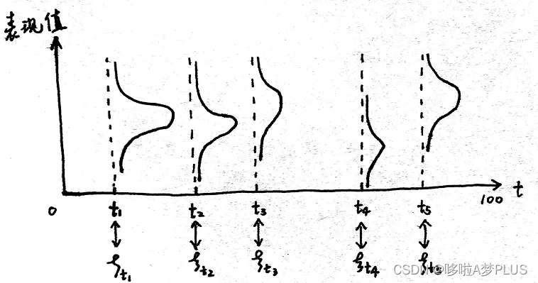
将多元高斯分布推广到连续域上的无限维高斯分布,就得到了高斯过程。如下图所示,在时域上,对于每一时刻
,相应的表观值都服从高斯分布,即是
,那么对于整个时域
上的联合分布,满足多元高斯分布,即是
其中每个时刻的均值用一个均值函数刻画,两个不同时刻之间的相关性用一个协方差函数刻画。
因此我们只需要两个因素来确定一个高斯过程:
- 均值函数
- 协方差函数(矩阵)
2.高斯过程回归
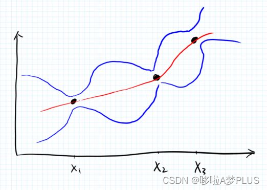
高斯过程回归的是通过有限的高维数据来拟合出相应的高斯过程,从而来预测任意随机变量下的函数值。具体而言,对于一组随机变量和目标值
,我们假设其服从多元高斯分布,即是:
这其中的问题是需要确定协方差矩阵,它反映了不同采样点之间的相似性大小,合法的协方差矩阵要求是半正定的,因此这里我们需要指定相应的核函数来度量这一相似性,sklearn中提供了很多的核函数,后面介绍。确定了协方差矩阵之后,我们就能根据已有的数据确定变量空间中的无限维高斯分布,并且相应地能够确定任意采样点处的条件高斯分布,即是相应的概率分布,如下图所示:
四、sklearn中高斯过程回归的使用
1. 核函数的选择
前面已经说明,核函数的作用是描述不同采样点之间的相似性大小,sklearn中内置了很多核函数,如下图所示:
Kernel which is composed of a set of other kernels. | |
Constant kernel. | |
Dot-Product kernel. | |
Exp-Sine-Squared kernel (aka periodic kernel). | |
The Exponentiation kernel takes one base kernel and a scalar parameter p and combines them via | |
A kernel hyperparameter's specification in form of a namedtuple. | |
Base class for all kernels. | |
Matern kernel. | |
Wrapper for kernels in sklearn.metrics.pairwise. | |
| The |
| Radial basis function kernel (aka squared-exponential kernel). |
Rational Quadratic kernel. | |
| The |
White kernel. |
除了sklearn中提供的核函数之外,也可以自定义核函数。
2. sklearn中高斯过程回归的使用
a. 初始数据
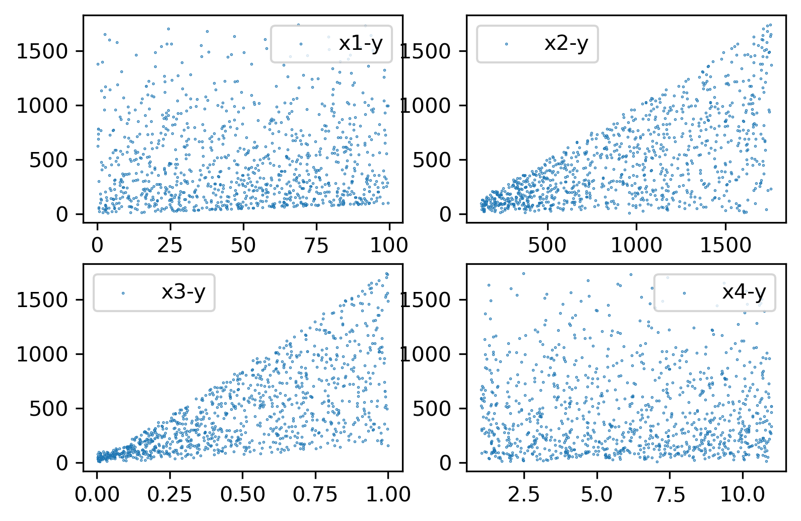
这里我们利用 sklearn.datasets.make_friedman2 生成初始数据,friedman2 生成输入数据是一个 n_sample x 4维的矩阵,下面是其调用及可视化。
from sklearn.datasets import make_friedman2
import matplotlib.pyplot as plt

X, y = make_friedman2(n_samples=1000, noise=0.1, random_state=10)

plt.figure(dpi=300)
ax1 = plt.subplot(221)
ax1.scatter(X[:, 0], y, label='x1-y', s=0.1)
ax1.legend()

ax1 = plt.subplot(222)
ax1.scatter(X[:, 1], y, label='x2-y', s=0.1)
ax1.legend()

ax1 = plt.subplot(223)
ax1.scatter(X[:, 2], y, label='x3-y', s=0.1)
ax1.legend()

ax1 = plt.subplot(224)
ax1.scatter(X[:, 3], y, label='x4-y', s=0.1)
ax1.legend()
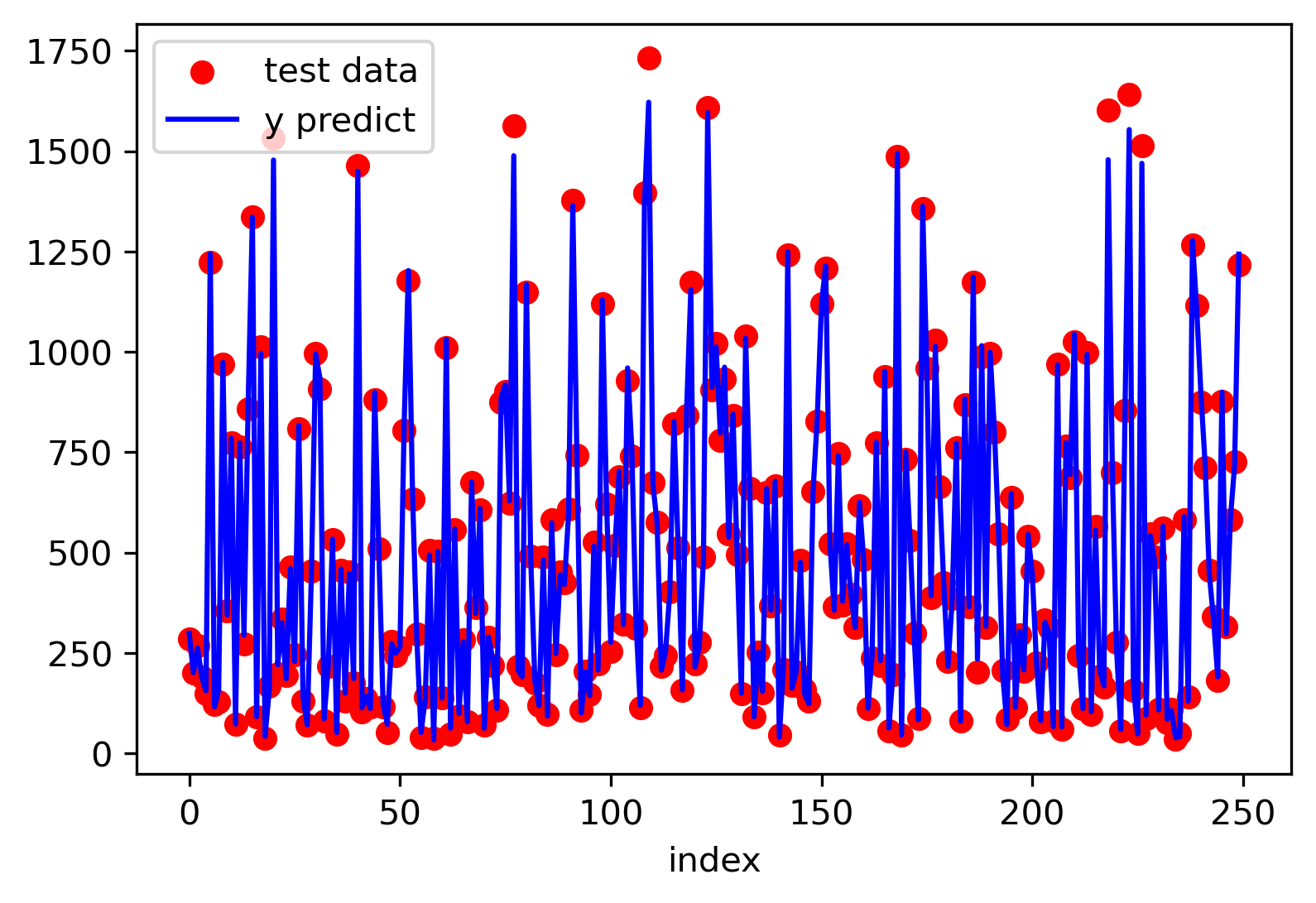
b. 高斯过程回归拟合
from sklearn.datasets import make_friedman2
from sklearn.model_selection import train_test_split
from sklearn.gaussian_process import GaussianProcessRegressor
from sklearn.gaussian_process.kernels import RBF, Sum, WhiteKernel
import matplotlib.pyplot as plt

X, y = make_friedman2(n_samples=1000, noise=0.1, random_state=10)

X_train, X_test, y_train, y_test = train_test_split(X, y, test_size=0.25, random_state=36)

model_kernel = Sum(RBF([100, 1500, 1, 10], length_scale_bounds='fixed'), WhiteKernel(0.1, noise_level_bounds='fixed'))

model_gpr = GaussianProcessRegressor(kernel=model_kernel)

model_gpr.fit(X_train, y_train)

print(model_gpr.score(X_test, y_test))

y_mean, y_std = model_gpr.predict(X_test, return_std=True)

plot_x = [i for i in range(X_test.shape[0])]
plt.figure(dpi=300)
plt.scatter(plot_x, y_test, color='red', label='test data')
plt.plot(plot_x, y_mean, color='blue', label='y predict')
plt.legend()
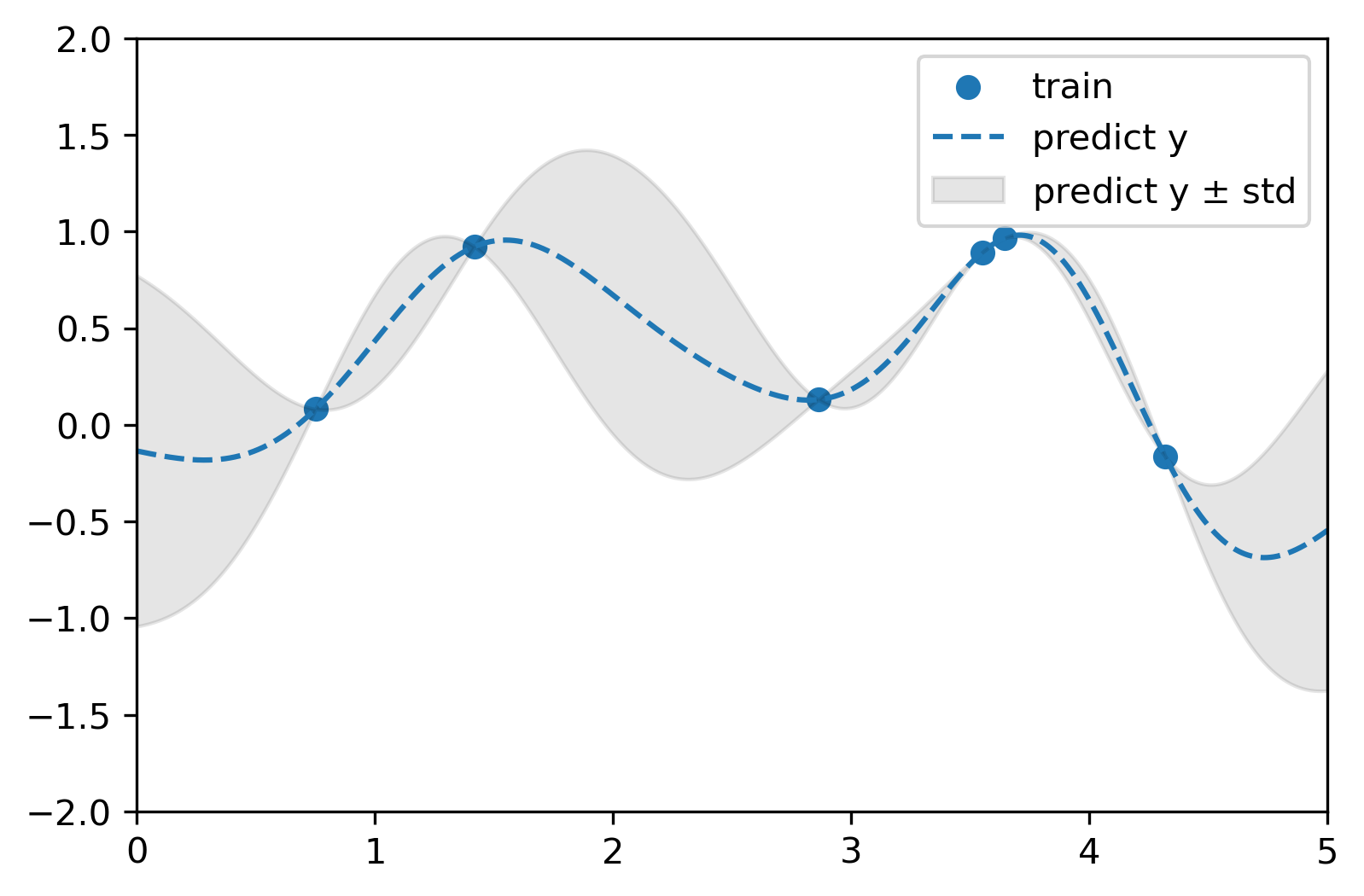
c. 高斯过程回归后验结果分布
from sklearn.datasets import make_friedman2
from sklearn.model_selection import train_test_split
from sklearn.gaussian_process import GaussianProcessRegressor
from sklearn.gaussian_process.kernels import DotProduct, RBF, Sum, Matern, PairwiseKernel
import matplotlib.pyplot as plt
import numpy as np

x_train = np.random.uniform(0, 5, 6).reshape(-1, 1)
y_train = np.sin(np.power(x_train-2.5, 2))

model_kernel = RBF(length_scale=1.0, length_scale_bounds=(1e-1, 10.0))
model_gpr = GaussianProcessRegressor(kernel=model_kernel)
model_gpr.fit(x_train, y_train)
plot_x = np.linspace(0, 5, 10000).reshape(-1, 1)
y_mean, y_std = model_gpr.predict(plot_x, return_std=True)
plt.figure(dpi=300)
plt.xlim([0, 5.0])
plt.ylim([-2.0, 2.0])
plt.scatter(x_train, y_train, label="train")
plt.plot(plot_x[:, 0], y_mean, '--', label='predict y')
plt.fill_between(plot_x[:, 0], y_mean-y_std, y_mean+y_std, color='black', alpha=0.1, label=r"predict y $\pm$ std")
plt.legend()
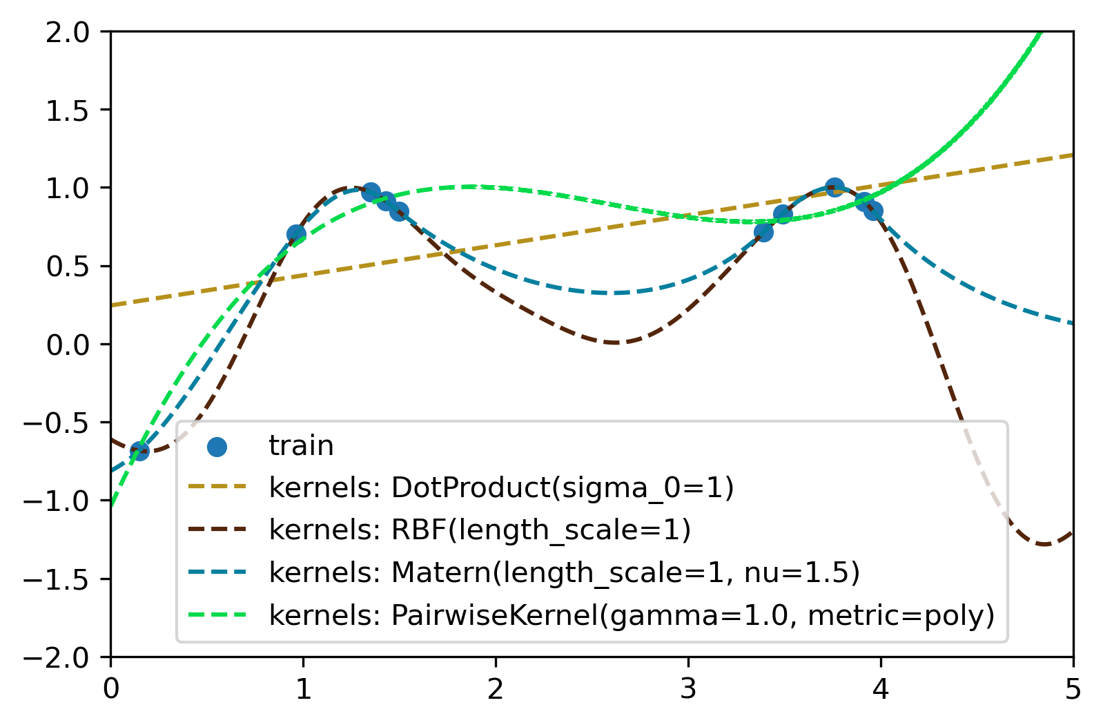
d. 不同核函数拟合结果对比
对于以上c中的数据,这里用了四种不同的核函数来拟合,如下为代码和拟合结果。
from sklearn.datasets import make_friedman2
from sklearn.model_selection import train_test_split
from sklearn.gaussian_process import GaussianProcessRegressor
from sklearn.gaussian_process.kernels import DotProduct, RBF, Matern, PairwiseKernel
import matplotlib.pyplot as plt
import numpy as np

x_train = np.random.uniform(0, 5, 10).reshape(-1, 1)
y_train = np.sin(np.power(x_train-2.5, 2))

model_k1 = DotProduct(sigma_0=1, sigma_0_bounds=(1e-1, 10.0))
model_k2 = RBF(length_scale=1.0, length_scale_bounds=(1e-1, 10.0))
model_k3 = Matern(length_scale=1.0, length_scale_bounds=(1e-1, 10.0), nu=1.5)
model_k4 = PairwiseKernel(gamma=1.0, gamma_bounds=(1e-1, 10), metric='poly')

plt.figure(dpi=300)
plt.xlim([0, 5.0])
plt.ylim([-2.0, 2.0])
plt.scatter(x_train, y_train, label="train")
plot_x = np.linspace(0, 5, 10000).reshape(-1, 1)

for model_kernel in [model_k1, model_k2, model_k3, model_k4]:
    model_gpr = GaussianProcessRegressor(kernel=model_kernel)
    model_gpr.fit(x_train, y_train)
    y_mean = model_gpr.predict(plot_x)
    plt.plot(plot_x[:, 0], y_mean, '--', color=(np.random.random(), np.random.random(), np.random.random()), label='kernels: {}'.format(model_kernel.__str__()))
plt.legend()
文章出处登录后可见!