接触PINN一段时间了,用深度学习的方法求解偏微分方程PDE,看来是非常不错的方法。做了一个简单易懂的例子,这个例子非常适合初学者。跟着教程做了一个小demo, 大家可以参考参考。本文代码亲测可用,直接复制就能使用,非常方便。
所用工具
使用了python和pytorch进行实现
python3.6
toch1.10
数学方程
使用一个最简单的偏微分方程:
要拟合的显示方程可以表示为
模型搭建
核心-使用最简单的全连接层:
class Net(nn.Module):
    def __init__(self, NN): # NL n个l(线性,全连接)隐藏层, NN 输入数据的维数, 128 256
        # NL是有多少层隐藏层
        # NN是每层的神经元数量
        super(Net, self).__init__()

        self.input_layer = nn.Linear(2, NN)
        self.hidden_layer1 = nn.Linear(NN,int(NN/2)) ## 原文这里用NN,我这里用的下采样,经过实验验证,“等采样”更优
        self.hidden_layer2 = nn.Linear(int(NN/2), int(NN/2)  ## 原文这里用NN,我这里用的下采样,经过实验验证,“等采样”更优
        self.output_layer = nn.Linear(int(NN/2, 1)

    def forward(self, x): # 一种特殊的方法 __call__() 回调
        out = torch.tanh(self.input_layer(x))
        out = torch.tanh(self.hidden_layer1(out))
        out = torch.tanh(self.hidden_layer2(out))
        out_final = self.output_layer(out)
        return out_final
偏微分方程定义,也就是公式(1):
def pde(x, net):
    u = net(x)  # 网络得到的数据
    u_tx = torch.autograd.grad(u, x, grad_outputs=torch.ones_like(net(x)),
                               create_graph=True, allow_unused=True)[0]  # 求偏导数
    d_t = u_tx[:, 0].unsqueeze(-1)
    d_x = u_tx[:, 1].unsqueeze(-1)
    u_xx = torch.autograd.grad(d_x, x, grad_outputs=torch.ones_like(d_x),
                               create_graph=True, allow_unused=True)[0][:,1].unsqueeze(-1)  # 求偏导数

    w = torch.tensor(0.01 / np.pi)

    return d_t + u * d_x - w * u_xx  # 公式(1)
所有实现代码
一下代码复制粘贴,可直接运行:
import torch
import torch.nn as nn
import torch
import torch.nn as nn
import numpy as np
import matplotlib.pyplot as plt
import torch.optim as optim
from torch.autograd import Variable
import numpy as np
from matplotlib import cm


# 模型搭建
class Net(nn.Module):
    def __init__(self, NN): # NL n个l(线性,全连接)隐藏层, NN 输入数据的维数, 128 256
        # NL是有多少层隐藏层
        # NN是每层的神经元数量
        super(Net, self).__init__()

        self.input_layer = nn.Linear(2, NN)
        self.hidden_layer1 = nn.Linear(NN,int(NN/2)) ## 原文这里用NN,我这里用的下采样,经过实验验证,“等采样”更优
        self.hidden_layer2 = nn.Linear(int(NN/2), int(NN/2))  ## 原文这里用NN,我这里用的下采样,经过实验验证,“等采样”更优
        self.output_layer = nn.Linear(int(NN/2, 1))

    def forward(self, x): # 一种特殊的方法 __call__() 回调
        out = torch.tanh(self.input_layer(x))
        out = torch.tanh(self.hidden_layer1(out))
        out = torch.tanh(self.hidden_layer2(out))
        out_final = self.output_layer(out)
        return out_final

def pde(x, net):
    u = net(x)  # 网络得到的数据
    u_tx = torch.autograd.grad(u, x, grad_outputs=torch.ones_like(net(x)),
                               create_graph=True, allow_unused=True)[0]  # 求偏导数
    d_t = u_tx[:, 0].unsqueeze(-1)
    d_x = u_tx[:, 1].unsqueeze(-1)
    u_xx = torch.autograd.grad(d_x, x, grad_outputs=torch.ones_like(d_x),
                               create_graph=True, allow_unused=True)[0][:,1].unsqueeze(-1)  # 求偏导数

    w = torch.tensor(0.01 / np.pi)

    return d_t + u * d_x - w * u_xx  # 公式(1)


net = Net(30)
mse_cost_function = torch.nn.MSELoss(reduction='mean')  # Mean squared error
optimizer = torch.optim.Adam(net.parameters(), lr=1e-4)


# 初始化 常量
t_bc_zeros = np.zeros((2000, 1))
x_in_pos_one = np.ones((2000, 1))
x_in_neg_one = -np.ones((2000, 1))
u_in_zeros = np.zeros((2000, 1))

iterations = 10000
for epoch in range(iterations):
    optimizer.zero_grad()  # 梯度归0

    # 求边界条件的误差
    # 初始化变量
    t_in_var = np.random.uniform(low=0, high=1.0, size=(2000, 1))
    x_bc_var = np.random.uniform(low=-1.0, high=1.0, size=(2000, 1))
    u_bc_sin = -np.sin(np.pi * x_bc_var)

    # 将数据转化为torch可用的
    pt_x_bc_var = Variable(torch.from_numpy(x_bc_var).float(), requires_grad=False)
    pt_t_bc_zeros = Variable(torch.from_numpy(t_bc_zeros).float(), requires_grad=False)
    pt_u_bc_sin = Variable(torch.from_numpy(u_bc_sin).float(), requires_grad=False)
    pt_x_in_pos_one = Variable(torch.from_numpy(x_in_pos_one).float(), requires_grad=False)
    pt_x_in_neg_one = Variable(torch.from_numpy(x_in_neg_one).float(), requires_grad=False)
    pt_t_in_var = Variable(torch.from_numpy(t_in_var).float(), requires_grad=False)
    pt_u_in_zeros = Variable(torch.from_numpy(u_in_zeros).float(), requires_grad=False)

    # 求边界条件的损失
    net_bc_out = net(torch.cat([pt_t_bc_zeros, pt_x_bc_var], 1))  # u(x,t)的输出
    mse_u_2 = mse_cost_function(net_bc_out, pt_u_bc_sin)  # e = u(x,t)-(-sin(pi*x))  公式(2)

    net_bc_inr = net(torch.cat([pt_t_in_var, pt_x_in_pos_one], 1))  # 0=u(t,1) 公式(3)
    net_bc_inl = net(torch.cat([pt_t_in_var, pt_x_in_neg_one], 1))  # 0=u(t,-1) 公式(4)

    mse_u_3 = mse_cost_function(net_bc_inr, pt_u_in_zeros)  # e = 0-u(t,1) 公式(3)
    mse_u_4 = mse_cost_function(net_bc_inl, pt_u_in_zeros)  # e = 0-u(t,-1) 公式(4)

    # 求PDE函数式的误差
    # 初始化变量
    x_collocation = np.random.uniform(low=-1.0, high=1.0, size=(2000, 1))
    t_collocation = np.random.uniform(low=0.0, high=1.0, size=(2000, 1))
    all_zeros = np.zeros((2000, 1))
    pt_x_collocation = Variable(torch.from_numpy(x_collocation).float(), requires_grad=True)
    pt_t_collocation = Variable(torch.from_numpy(t_collocation).float(), requires_grad=True)
    pt_all_zeros = Variable(torch.from_numpy(all_zeros).float(), requires_grad=False)

    # 将变量x,t带入公式(1)
    f_out = pde(torch.cat([pt_t_collocation, pt_x_collocation], 1), net)  # output of f(x,t) 公式(1)
    mse_f_1 = mse_cost_function(f_out, pt_all_zeros)

    # 将误差(损失)累加起来
    loss = mse_f_1 + mse_u_2 + mse_u_3 + mse_u_4

    loss.backward()  # 反向传播
    optimizer.step()  # This is equivalent to : theta_new = theta_old - alpha * derivative of J w.r.t theta

    with torch.autograd.no_grad():
        if epoch % 100 == 0:
            print(epoch, "Traning Loss:", loss.data)

## 画图 ##
t = np.linspace(0, 1, 100)
x = np.linspace(-1, 1, 256)
ms_t, ms_x = np.meshgrid(t, x)
x = np.ravel(ms_x).reshape(-1, 1)
t = np.ravel(ms_t).reshape(-1, 1)
pt_x = Variable(torch.from_numpy(x).float(), requires_grad=True)
pt_t = Variable(torch.from_numpy(t).float(), requires_grad=True)
pt_u0 = net(torch.cat([pt_t, pt_x], 1))
u = pt_u0.data.cpu().numpy()

pt_u0 = u.reshape(256, 100)

fig = plt.figure()
ax = fig.add_subplot(projection='3d')
ax.set_zlim([-1, 1])
ax.plot_surface(ms_t, ms_x, pt_u0, cmap=cm.RdYlBu_r, edgecolor='blue', linewidth=0.0003, antialiased=True)
ax.set_xlabel('t')
ax.set_ylabel('x')
ax.set_zlabel('u')
plt.savefig('Preddata.png')
plt.close(fig)
结果展示
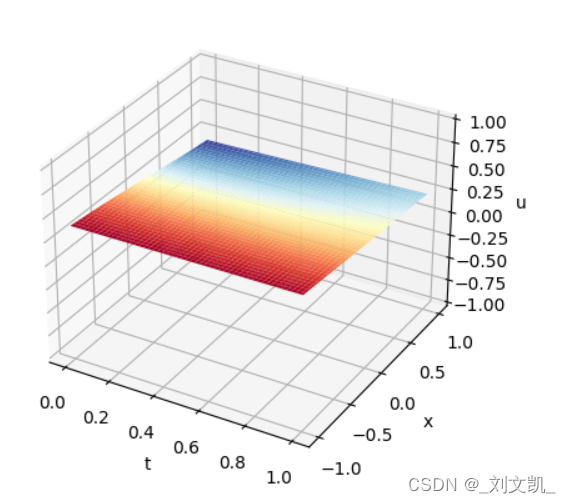
训练0次时的结果也就是没训练,下面为模拟值:
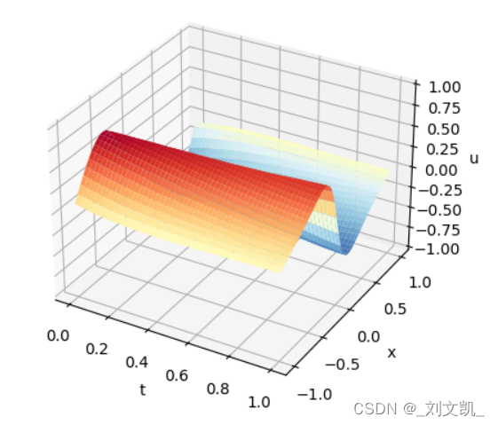
训练10000时的结果:
参考文献
[1]. 每天进步一点点吧. PINN学习记录.
https://blog.csdn.net/weixin_45805559/article/details/121574293
文章出处登录后可见!
已经登录?立即刷新