🗺 🌏Cartopy地图绘图包——“专为地理空间数据处理而设计,以生成地图和其他地理空间数据分析。”,是在PROJ、pyshp、shapely、GEOS等Python包的基础上编写的,在安装时,需要同时安装相关的依赖包。
🌎Cartopy包对Matplotlib包的功能进行了扩展,两者结合使用能绘制各种地图。详情介绍可访问官网:https://scitools.org.uk/cartopy/docs/latest/index.html
🗺
1、Cartopy包的安装
①通过pip来下载安装,在cmd命令行下输入pip install cartopy,可直接下载安装cartopy及其依赖包。
②在编辑器PyCharm中下载安装:
注:在首先下载时,我用Python的是3.10版本,下载失败了。后面我就先把一些依赖包提前下载好,再去下载cartopy包依然没成功。后面参考了这篇文章:博客【在Python下载cartopy库以及地图文件存放的问题】,换用python3.9.7的环境来下载安装cartopy包,成功了!
2、Cartopy包基础学习
1.坐标参考系
地图绘制涉及坐标参考系(coordinate reference system,crs),同个数据,采用不同坐标参考系统绘制的地图是不同的。
cartopy包中的crs模块定义了20多个常用的坐标参考系统类(利用proj包),用于创建不同的crs对象。
【PS:PROJ.4是开源GIS最著名的地图投影库,它专注于地图投影的表达,以及转换,许多GIS开源软件的投影都直接使用Proj.4的库文件。https://www.osgeo.cn/pygis/proj-projintro.html】
cartopy定义的主要坐标参照系统类
| 坐标参照系统类 | 解释 |
|---|---|
| PlateCarree | 把经纬度的值作为x,y坐标值 |
| AlbersEqualArea | 阿伯斯等积圆锥投影 |
| LambertConformal | 兰伯特等角圆锥投影 |
| Mercator | 墨卡托投影(正轴圆柱投影) |
| UTM | 通用横轴墨卡托投影(分带投影) |
同时,在创建坐标参照系统对象时,可以通过关键字参数设置坐标参照系统参数。常用的关键字参数有:
- central_longitude(中央经线)
- central_latitude(中央纬线)
- standard_parallels(标准纬线)
- globe(大地测量基准)
创建crs对象的一些示例:
cartopy.crs.PlateCarree(central_longitude=180)
cartopy.crs.LambertConformal(central_longitude=110)
cartopy.crs.AlbersEqualArea(central_longitude=105.0, standard_parallels=(25.0, 45.0))
cartopy.crs.UTM(zone=30)
2.加载空间数据
绘制前提(Geoaxes对象的创建):
当创建绘图区域(axes类)时,可以定义projection关键字参数。当projection关键字参数的值是crs对象时,这是返回的对象是Geoaxes对象。
如:
fig = plt.figure()  # 创建Figure对象
crs = ccrs.PlateCarree()  # 创建crs对象
ax = fig.add_subplot(2, 1, 1, projection=crs)  # 通过添加projection参数 创建geoaxes对象
print(ax)
'''返回:< GeoAxes: <cartopy.crs.PlateCarree object at 0x000002AE4C56AB80> >'''
Geoaxes是特殊的axes对象,能按指定的坐标系统加载绘制不同形式的空间坐标数据。
加载数据:
下面是Geoaxes对象支持加载的一些数据:
(1)Natural Earth共享数据网站上的开放数据。
- coastlines() 方法,从Natural Earth网站加载coastline数据,可通过resolution关键字参数指定加载数据的比例尺(目前有110m、50m和10m,缺省则为110m。这里的m是million)
- stock_img() 方法,从Natural Earth网站加载晕渲地形栅格数据。
- 此外,Natural Earth网站上的其他数据集可以通过cartopy.feature.NaturalEarthFeature构造函数产生Feature对象,然后利用Geoaxes对象的add_feature()方法进行加载。
- 为了方便操作,cartopy预定义了Natural Earth网站上的一些数据集。我们也可以自己去将数据下载到本地,官网:https://www.naturalearthdata.com/
(2)shapely包定义的Geometries对象数据。
- add_geometries(geoms, crs) 方法,加载指定crs的Geometries对象数据。
- 另外,通过io模块中的shapereader函数可以读取 Esri 的 shapefile数据,然后转换成Geometries对象进行加载。
(3)wms(Web地图服务)和wmts(Web地图切片服务)数据。
- add_wms()方法,加载wms(Web地图服务)数据, 参数wms设置要使用的 web 地图服务 URL 或 owslib WMS 实例,参数layers设置调用的图层名称。
- add_wmts()方法,加载wmts(Web地图切片服务)数据,参数wmts设置服务的URL,参数layer_name设置调用的图层名称。
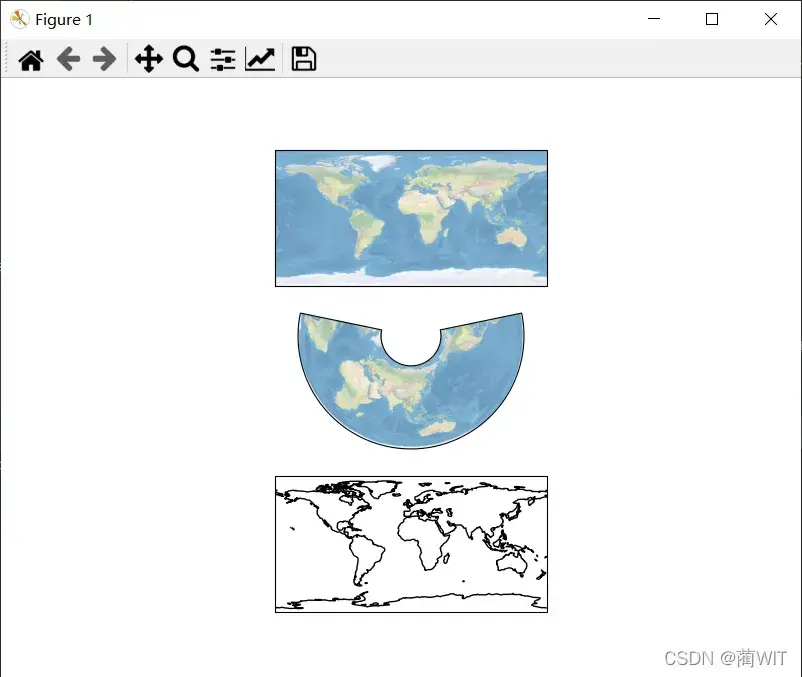
示例(1):在不同坐标系下绘制Natural Earth共享数据网站上的地图数据
代码及注释:
import matplotlib.pyplot as plt
import cartopy.crs as ccrs

fig = plt.figure(figsize=(8, 6))

crs = ccrs.PlateCarree()
ax = fig.add_subplot(3, 1, 1, projection=crs)
ax.stock_img()  # 加载地理坐标系统下的全球晕渲地形图

crs = ccrs.AlbersEqualArea(central_longitude=105.0, standard_parallels=(25.0, 45.0))
ax = fig.add_subplot(3, 1, 2, projection=crs)
ax.stock_img()  # 加载阿伯斯等积投影坐标系统下的全球晕渲地形图

ax = fig.add_subplot(3, 1, 3, projection=ccrs.PlateCarree())
ax.coastlines()  # 加载地理坐标系统下的全球海陆边界线地图
plt.show()
效果图:
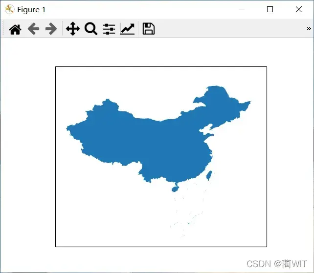
示例(2):利用shape矢量数据来加载地理坐标系下的中国国界图
代码及注释:
import matplotlib.pyplot as plt
import cartopy.crs as ccrs
import cartopy.io.shapereader as sr

fig = plt.figure()
crs = ccrs.PlateCarree()
ax = fig.add_subplot(1, 1, 1, projection=crs)
geom = sr.Reader("D:/tmp/shapedata/中国国界.shp").geometries()  # 读取shapefile数据,转换成Geometries对象进行加载
ax.add_geometries(geom, crs)  # 将Geometries对象数据加载到绘图区域
ax.set_extent((70, 140, 0, 60), crs)  # 设置指定坐标系下的地图显示范围
plt.show()
效果图:
示例(3):加载arcgisonline提供的网络地图服务数据
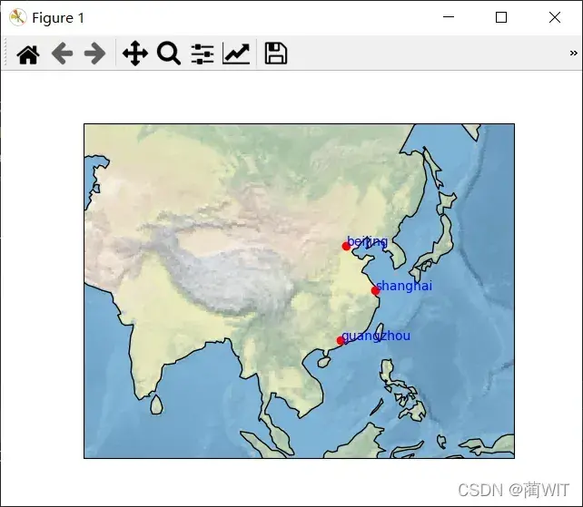
示例:把点数据叠置在不同坐标参照系统的背景地图上
( 在利用plot()绘制点图时,如果点数据和绘图区域的坐标系统不一致,可以定义关键字参数transform的值为数据的crs对象,即可将点数据转换成绘图区域坐标值 )
代码:
import matplotlib.pyplot as plt
import cartopy.crs as ccrs

crs = ccrs.AlbersEqualArea(central_longitude=105.0, standard_parallels=(25.0, 45.0))
ax = plt.axes(projection=crs)
ax.coastlines(resolution='110m')
ax.stock_img()
x_list = [116.37, 121.53, 113.25]
y_list = [39.92, 31.26, 23.13]
city = ["beijing", "shanghai", "guangzhou"]
data_crs = ccrs.PlateCarree()
plt.plot(x_list, y_list, "o", color="r", markersize=6, transform=data_crs)  # 绘制点
for i in range(len(city)):
    plt.text(x_list[i], y_list[i], city[i], transform=data_crs, color="b")  # 添加点的标注
ax.set_extent((70, 140, 0, 60), ccrs.PlateCarree())
plt.show()
效果图:
3.绘制网格线
Geoaxes对象的gridlines()方法用于绘制网格线,该方法返回一个Gridliner对象,通过对Gridliner对象属性设置,可以绘制不同形式的网格线。
网格线的一些相关属性:
- xlines和ylines,x和y轴是否画线;
- xlocator和ylocation,画线的位置;
- xlabels_top、xlabels_bottom、xlabels_left、xlabels_right,标注的位置;
- xformatter和yformatter,标注的格式。(这里 cartopy.mpl.gridliner定义了LONGITUDE_FORMATTER和LATITUDE_FORMATTER两个类,用于产生格式化的经纬度标注。)
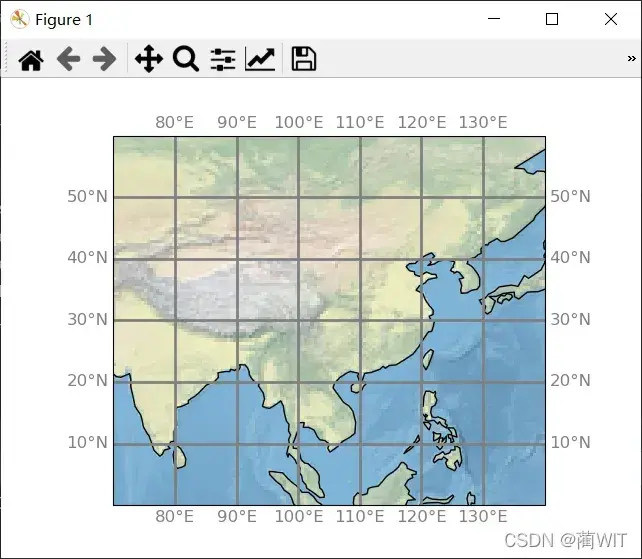
示例:绘制中国区域的网格线及其标注
代码:
import matplotlib.pyplot as plt
import matplotlib.ticker as mticker
import cartopy.feature
import cartopy.crs as ccrs
from cartopy.mpl.gridliner import LATITUDE_FORMATTER, LONGITUDE_FORMATTER

ax = plt.axes(projection=ccrs.PlateCarree())
ax.coastlines()
ax.stock_img()
ax.set_extent((70, 140, 0, 60), ccrs.PlateCarree())
gl = ax.gridlines(crs=ccrs.PlateCarree(), draw_labels=True, linewidth=2, color='gray')
gl.xlocator = mticker.FixedLocator([70, 80, 90, 100, 110, 120, 130, 140])
gl.ylocator = mticker.FixedLocator([0, 10, 20, 30, 40, 50, 60])
gl.xformartter = LONGITUDE_FORMATTER
gl.yformartter = LATITUDE_FORMATTER
gl.xlabel_style = {'size': 12, 'color': 'gray'}
gl.ylabel_style = {'size': 12, 'color': 'gray'}
plt.show()
效果图:
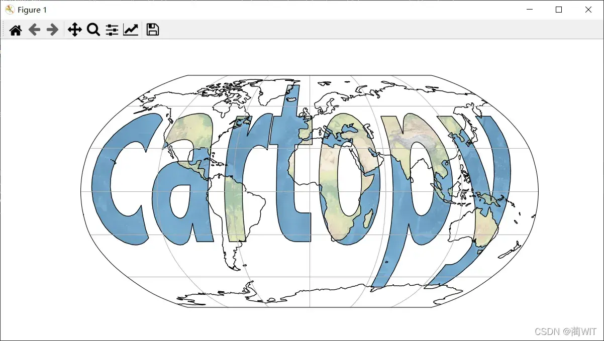
3、官网绘制示例
下面从官网:https://scitools.org.uk/cartopy/docs/latest/gallery/index.html上找了一些有趣的地图绘制例子。官网给出的示例,都是比较清晰健壮的代码编写出来的,感兴趣的朋友也可以自己分析研读一下,为自己制图培养一些技巧与灵感。😀
示例一:
import cartopy.crs as ccrs
import matplotlib.pyplot as plt
import matplotlib.textpath
import matplotlib.patches
from matplotlib.font_manager import FontProperties
import numpy as np

fig = plt.figure(figsize=[12, 6])
ax = fig.add_subplot(1, 1, 1, projection=ccrs.Robinson())

ax.coastlines()
ax.gridlines()

# generate a matplotlib path representing the word "cartopy"
fp = FontProperties(family='Bitstream Vera Sans', weight='bold')
logo_path = matplotlib.textpath.TextPath((-175, -35), 'cartopy',
                                         size=1, prop=fp)
# scale the letters up to sensible longitude and latitude sizes
logo_path._vertices *= np.array([80, 160])

# add a background image
im = ax.stock_img()
# clip the image according to the logo_path. mpl v1.2.0 does not support
# the transform API that cartopy makes use of, so we have to convert the
# projection into a transform manually
plate_carree_transform = ccrs.PlateCarree()._as_mpl_transform(ax)
im.set_clip_path(logo_path, transform=plate_carree_transform)

 # add the path as a patch, drawing black outlines around the text
patch = matplotlib.patches.PathPatch(logo_path,
                                      facecolor='none', edgecolor='black',
                                      transform=ccrs.PlateCarree())
ax.add_patch(patch)

plt.show()
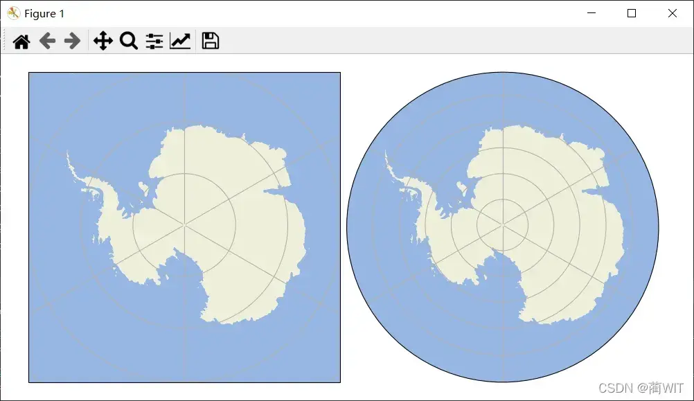
示例二:
import matplotlib.path as mpath
import matplotlib.pyplot as plt
import numpy as np

import cartopy.crs as ccrs
import cartopy.feature as cfeature


def main():
    fig = plt.figure(figsize=[10, 5])
    ax1 = fig.add_subplot(1, 2, 1, projection=ccrs.SouthPolarStereo())
    ax2 = fig.add_subplot(1, 2, 2, projection=ccrs.SouthPolarStereo(),
                          sharex=ax1, sharey=ax1)
    fig.subplots_adjust(bottom=0.05, top=0.95,
                        left=0.04, right=0.95, wspace=0.02)

    # Limit the map to -60 degrees latitude and below.
    ax1.set_extent([-180, 180, -90, -60], ccrs.PlateCarree())

    ax1.add_feature(cfeature.LAND)
    ax1.add_feature(cfeature.OCEAN)

    ax1.gridlines()
    ax2.gridlines()

    ax2.add_feature(cfeature.LAND)
    ax2.add_feature(cfeature.OCEAN)

    # Compute a circle in axes coordinates, which we can use as a boundary
    # for the map. We can pan/zoom as much as we like - the boundary will be
    # permanently circular.
    theta = np.linspace(0, 2*np.pi, 100)
    center, radius = [0.5, 0.5], 0.5
    verts = np.vstack([np.sin(theta), np.cos(theta)]).T
    circle = mpath.Path(verts * radius + center)

    ax2.set_boundary(circle, transform=ax2.transAxes)

    plt.show()


if __name__ == '__main__':
    main()
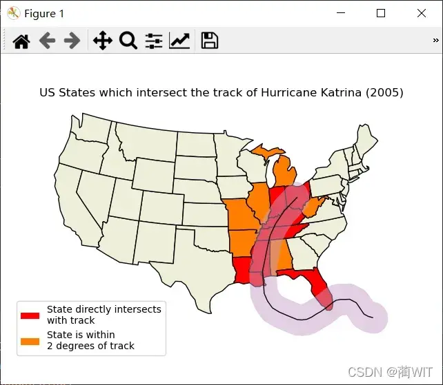
示例三:
import matplotlib.patches as mpatches
import matplotlib.pyplot as plt
import shapely.geometry as sgeom

import cartopy.crs as ccrs
import cartopy.io.shapereader as shpreader


def sample_data():
    """
    Return a list of latitudes and a list of longitudes (lons, lats)
    for Hurricane Katrina (2005).

    The data was originally sourced from the HURDAT2 dataset from AOML/NOAA:
    https://www.aoml.noaa.gov/hrd/hurdat/newhurdat-all.html on 14th Dec 2012.

    """
    lons = [-75.1, -75.7, -76.2, -76.5, -76.9, -77.7, -78.4, -79.0,
            -79.6, -80.1, -80.3, -81.3, -82.0, -82.6, -83.3, -84.0,
            -84.7, -85.3, -85.9, -86.7, -87.7, -88.6, -89.2, -89.6,
            -89.6, -89.6, -89.6, -89.6, -89.1, -88.6, -88.0, -87.0,
            -85.3, -82.9]

    lats = [23.1, 23.4, 23.8, 24.5, 25.4, 26.0, 26.1, 26.2, 26.2, 26.0,
            25.9, 25.4, 25.1, 24.9, 24.6, 24.4, 24.4, 24.5, 24.8, 25.2,
            25.7, 26.3, 27.2, 28.2, 29.3, 29.5, 30.2, 31.1, 32.6, 34.1,
            35.6, 37.0, 38.6, 40.1]

    return lons, lats


def main():
    fig = plt.figure()
    # to get the effect of having just the states without a map "background"
    # turn off the background patch and axes frame
    ax = fig.add_axes([0, 0, 1, 1], projection=ccrs.LambertConformal(),
                      frameon=False)
    ax.patch.set_visible(False)

    ax.set_extent([-125, -66.5, 20, 50], ccrs.Geodetic())

    shapename = 'admin_1_states_provinces_lakes'
    states_shp = shpreader.natural_earth(resolution='110m',
                                         category='cultural', name=shapename)

    lons, lats = sample_data()

    ax.set_title('US States which intersect the track of '
                 'Hurricane Katrina (2005)')

    # turn the lons and lats into a shapely LineString
    track = sgeom.LineString(zip(lons, lats))

    # buffer the linestring by two degrees (note: this is a non-physical
    # distance)
    track_buffer = track.buffer(2)

    def colorize_state(geometry):
        facecolor = (0.9375, 0.9375, 0.859375)
        if geometry.intersects(track):
            facecolor = 'red'
        elif geometry.intersects(track_buffer):
            facecolor = '#FF7E00'
        return {'facecolor': facecolor, 'edgecolor': 'black'}

    ax.add_geometries(
        shpreader.Reader(states_shp).geometries(),
        ccrs.PlateCarree(),
        styler=colorize_state)

    ax.add_geometries([track_buffer], ccrs.PlateCarree(),
                      facecolor='#C8A2C8', alpha=0.5)
    ax.add_geometries([track], ccrs.PlateCarree(),
                      facecolor='none', edgecolor='k')

    # make two proxy artists to add to a legend
    direct_hit = mpatches.Rectangle((0, 0), 1, 1, facecolor="red")
    within_2_deg = mpatches.Rectangle((0, 0), 1, 1, facecolor="#FF7E00")
    labels = ['State directly intersects\nwith track',
              'State is within \n2 degrees of track']
    ax.legend([direct_hit, within_2_deg], labels,
              loc='lower left', bbox_to_anchor=(0.025, -0.1), fancybox=True)

    plt.show()


if __name__ == '__main__':
    main()
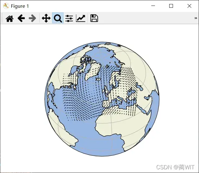
示例四:
import matplotlib.pyplot as plt
import numpy as np

import cartopy.crs as ccrs
import cartopy.feature as cfeature


def sample_data(shape=(20, 30)):
    """
    Return ``(x, y, u, v, crs)`` of some vector data
    computed mathematically. The returned crs will be a rotated
    pole CRS, meaning that the vectors will be unevenly spaced in
    regular PlateCarree space.

    """
    crs = ccrs.RotatedPole(pole_longitude=177.5, pole_latitude=37.5)

    x = np.linspace(311.9, 391.1, shape[1])
    y = np.linspace(-23.6, 24.8, shape[0])

    x2d, y2d = np.meshgrid(x, y)
    u = 10 * (2 * np.cos(2 * np.deg2rad(x2d) + 3 * np.deg2rad(y2d + 30)) ** 2)
    v = 20 * np.cos(6 * np.deg2rad(x2d))

    return x, y, u, v, crs


def main():
    fig = plt.figure()
    ax = fig.add_subplot(1, 1, 1, projection=ccrs.Orthographic(-10, 45))

    ax.add_feature(cfeature.OCEAN, zorder=0)
    ax.add_feature(cfeature.LAND, zorder=0, edgecolor='black')

    ax.set_global()
    ax.gridlines()

    x, y, u, v, vector_crs = sample_data()
    ax.quiver(x, y, u, v, transform=vector_crs)

    plt.show()


if __name__ == '__main__':
    main()
文章出处登录后可见!