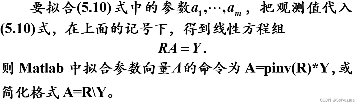
拟合
线性最小二乘法
1、解线性方程组 拟合参数
1、对于方程 y=a*t+b
clc, clear, t=[0:7]';
y=[27.0, 26.8, 26.5, 26.3, 26.1, 25.7, 25.3, 24.8]';
tb=mean(t); yb=mean(y);
ahat=sum((t-tb).*(y-yb))/sum((t-tb).^2) %编程计算
bhat=yb-ahat*tb
%以上是解方程得出的参数结果,以下是拟合得到的参数结果
R=[t,ones(8,1)];
cs=R\y  %解超定线性方程组求拟合参数 y=a*t+b
2、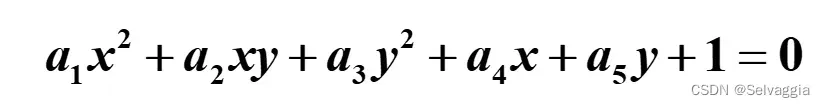
clc, clear
x0=[5.764  6.286  6.759  7.168  7.408]';
y0=[0.648  1.202  1.823  2.526  3.360]';
a=[x0.^2, x0.*y0, y0.^2, x0, y0];
b=-ones(5,1); c=a\b
fxy=@(x,y)c(1)*x.^2+c(2)*x.*y+c(3)*y.^2+c(4)*x+c(5)*y+1; %定义匿名函数
% h=fimplicit(fxy,[3.5,8,-1,5]), title('')
%fimplicit效果据说优于ezplot,但这里用不了,差不多啦
h=ezplot(fxy,[3.5,8,-1,5]), title('') %绘制隐函数、符号函数
set(h,'Color','k','LineWidth',1.5)
xlabel('$x$','Interpreter','Latex')
ylabel('$y$','Interpreter','Latex','Rotation',0)
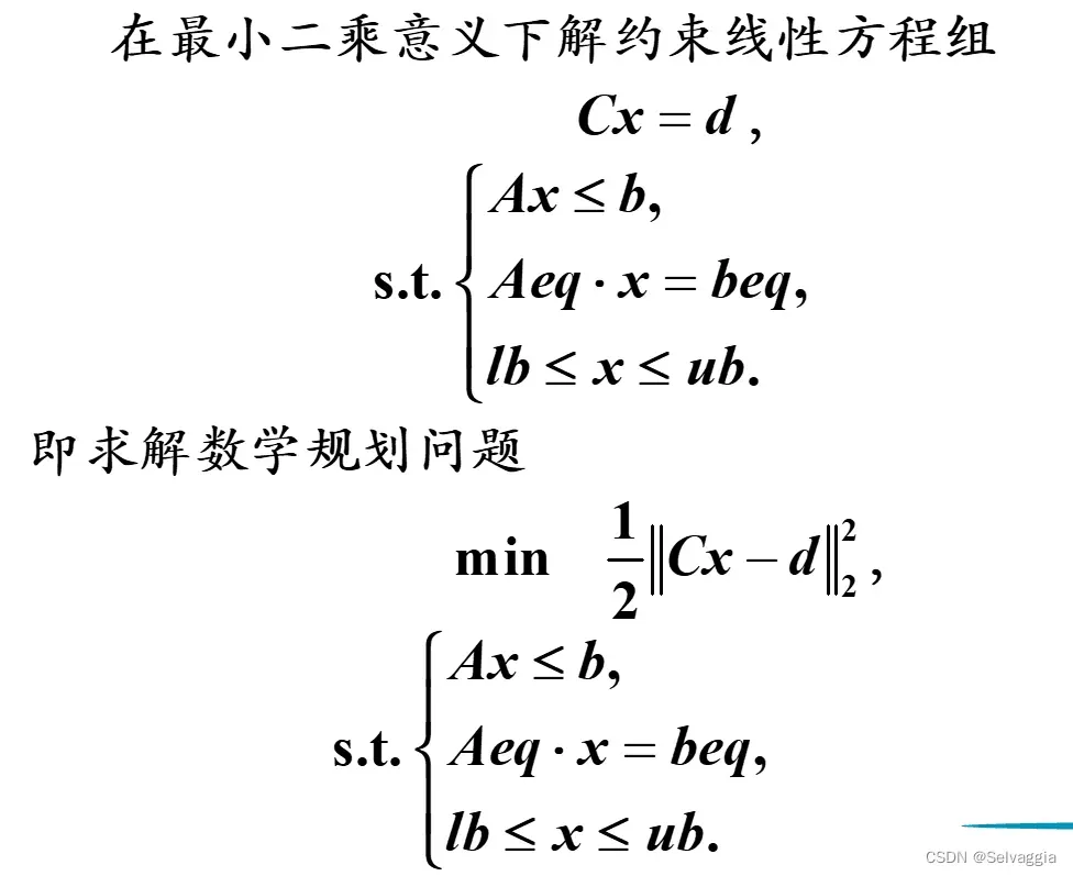
约束线性最小二乘解(解 约束线性方程组)
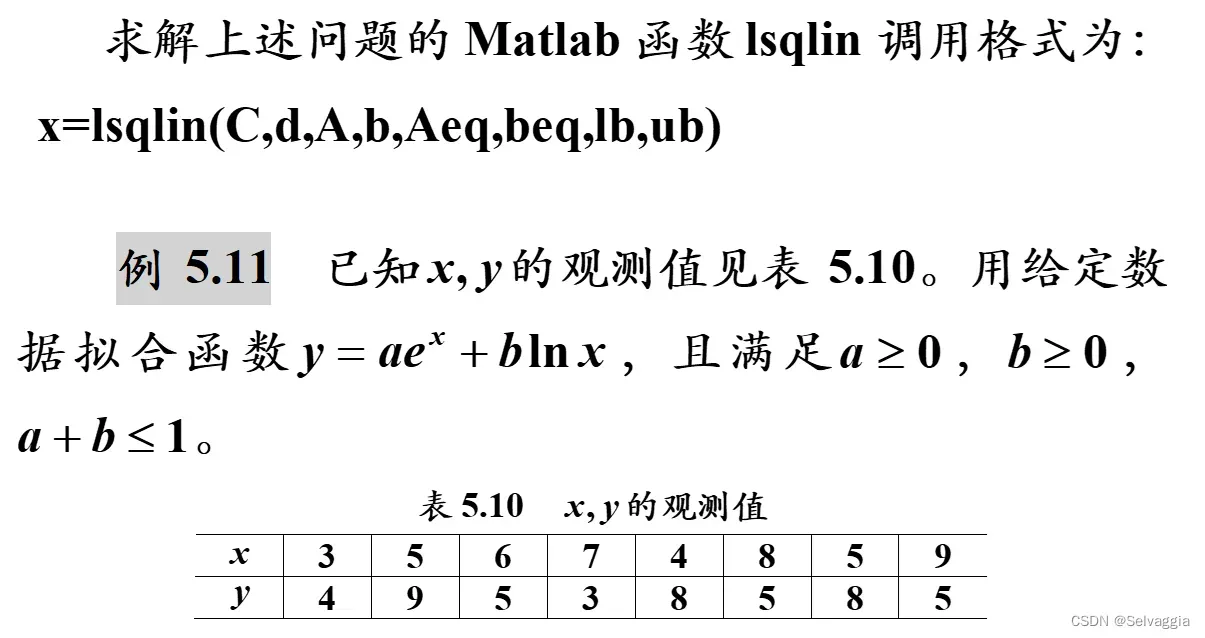
clc, clear, a=load('data5_11.txt');
x0=a(1,:)'; d=a(2,:)'; C=[exp(x0),log(x0)];
A=[1 1]; b=1; %线性不等式的约束矩阵和常数项列 A对应系数,b对应等式右侧值 a+b<=1
lb=zeros(2,1); %参数向量的下界
cs=lsqlin(C,d,A,b,[],[],lb) %拟合参数
多项式拟合
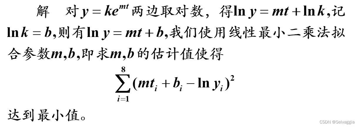
m、t为未知参数
clc, clear, a=load('data5_12.txt');
t0=a(1,:); y0=log(a(2,:));
p=polyfit(t0,y0,1), p(2)=exp(p(2))
原来ployfit还可以拟合像 lny=mx+b(这也是多项式?)这样的式子
fit 和fittype
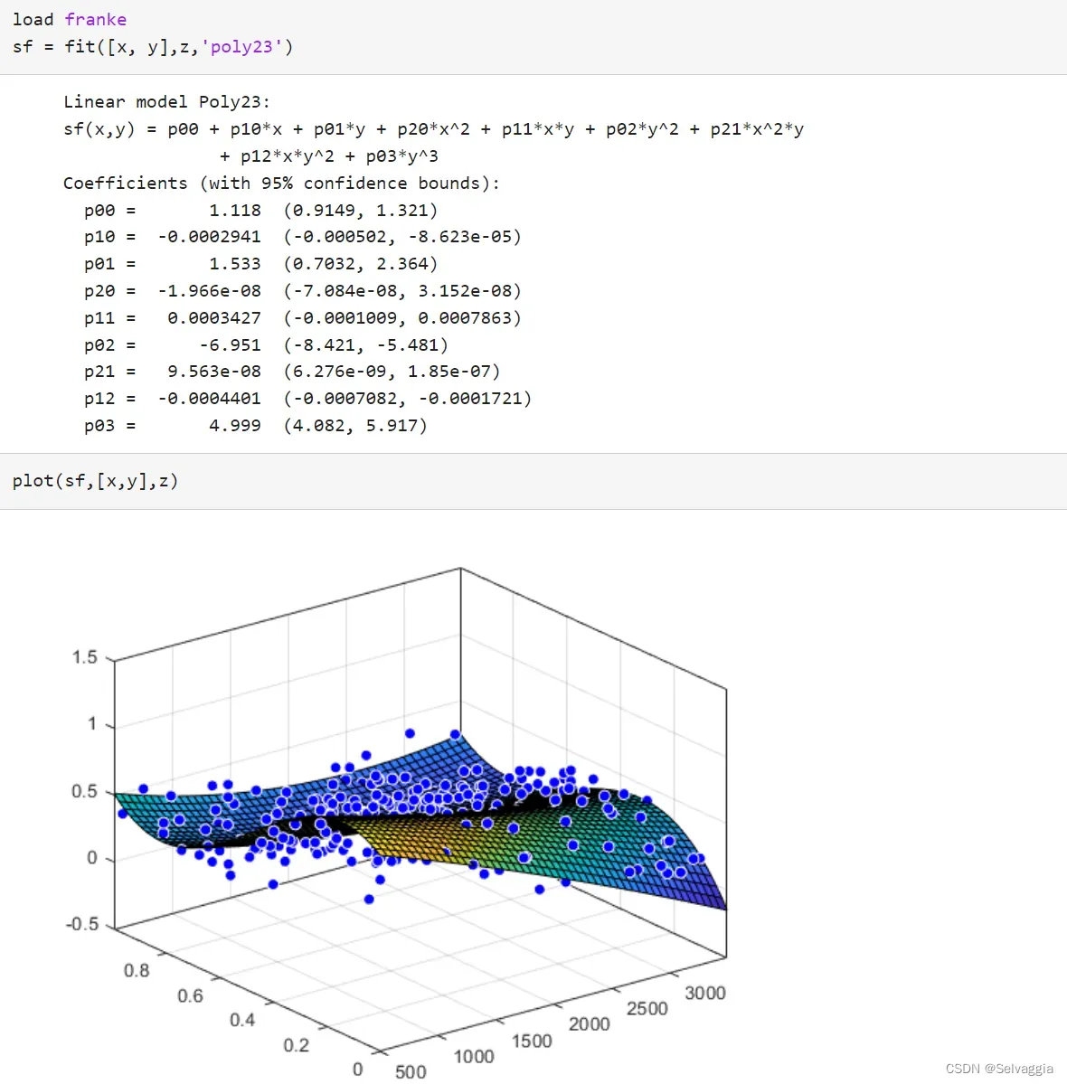
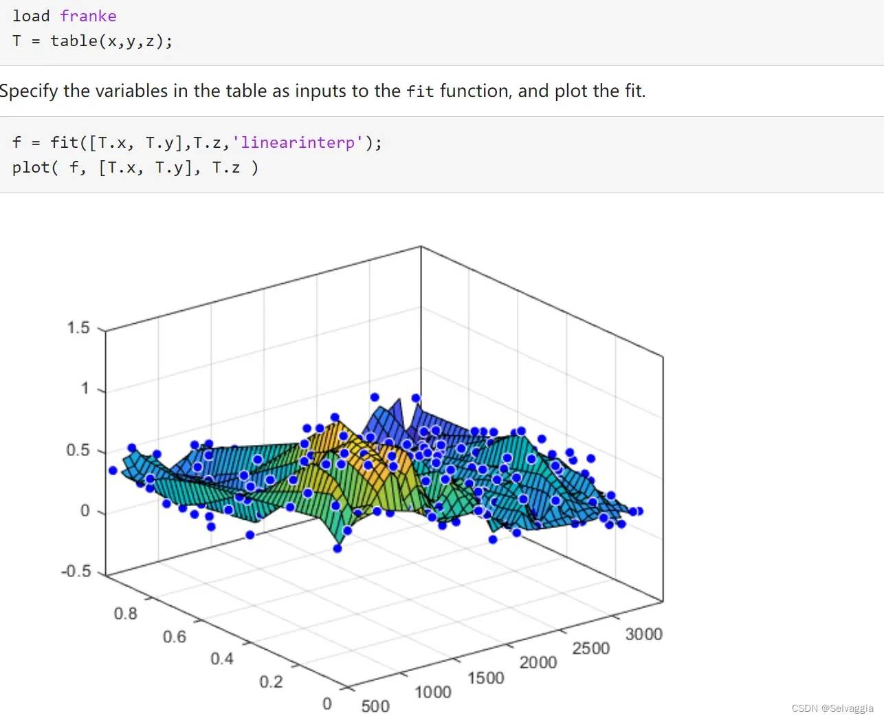
使用如下两种方式,可以使用MATLAB已经实现的拟合算法或者使用自定义的拟合算法(可以引用.m文件),具体算法有‘poly11’,‘poly2’,‘linearinterp’等,具体详见fittype的文档说明。
1、f = fittype(libraryModelName) %利用库模型函数类
f = fittype( 'gauss1' ); %高斯拟合
f=fit(t,y,'poly1') %利用库模型函数类
2、f = fittype(expression) %自定义函数
2.1 匿名函数
ft = fittype(@(a,b,c,x) a*x^3 + b*x^2 +c*x );
2.2 公式具体表达(常用)
f=fittype('公式具体表达','dependent','因变量名','independent','自变量名','coefficients',{'待定参数1','待定参数2'});

syms t;
x=[50; 200; 400; 600; 800];
y=[0.00000209; 0.00000267; 0.00000825; 0.000748; 0.0216];

f=fittype('C*(1-(0.0005)^(0.00013-0.000000372*t+0.0000000036*t^2))^(n+1)','independent','t','coefficients',{'C','n'});

[cfun,rsquare]=fit(x,y,f,'Lower',[580,1.4],'Upper',[3000000,3],'StartPoint',[600, 1.5]);


xi=0:1:850;
yi=cfun(xi);

plot(x,y,'r*',xi,yi,'b-');
clc, clear
x0=linspace(1,10,20); y0=linspace(3,20,20);
z0=1+2*log(x0)+3*y0;  %产生z=1+2lnx+3y的数据
g=fittype('a+b*log(x)+c*y', 'dependent', {'z'}, 'independent', {'x', 'y'})
f=fit([x0',y0'],z0',g,'StartPoint',rand(1,3))  %利用模拟数据拟合
fit
fitobject = fit(x,y,fitType)
fitobject = fit([x,y],z,fitType)
fitobject = fit(x,y,fitType,fitOptions)
fitobject = fit(x,y,fitType,Name,Value)
[fitobject,gof] = fit(x,y,fitType)
[fitobject,gof,output] = fit(x,y,fitType)
fitresult= fit( xData, yData, ftype);
其输出fitresult是一个cfit型的对象(object),主要包含两个内容:
1,拟合模型,即第一步中确定的拟合类型;
(即恰当的拟合函数,比如 f(x) = p1x + p2, fo(x) = a1exp(-((x-b1)/c1)^2)
2,拟合所得系数的值。例如对第一步中所创建的高斯模型,其fitresult 的值为
fitresult =
     General model Gauss1:
     fo(x) =  a1*exp(-((x-b1)/c1)^2)
     Coefficients (with 95% confidence bounds):
       a1 =       45.54  (42.45, 48.64)
       b1 =     0.01011  (0.0101, 0.01012)
       c1 =   0.0002551  (0.0002353, 0.0002748)
3、获得了这样一个object,如何把其中的系数提取出来呢?这个要用到coeffvalues函数
coeffvalues(fitresult)
ans =

   45.5426    0.0101    0.0003
4、获取拟合优度gof
现在已经获得了拟合系数,那到底拟合得怎么样呢?可以使用下面的格式获取拟合优度
[fitresult ,gof] = fit(X,Y,‘gauss1’);
gof是一个结构体,包含4个量
sse:Sunm of squares due to error
rsquare:R-square 这个就是线性回归里的那个R2,与线性回归里的具有同样的意义
dfe:Degrees of freedom in the error,不懂
adjrsquare: 也不懂
rmse: 误差的均方根值(rms)
接下来这个例子解释fit的具体用法
syms t;
x=[50; 200; 400; 600; 800];
y=[0.00000209; 0.00000267; 0.00000825; 0.000748; 0.0216];

f=fittype('C*(1-(0.0005)^(0.00013-0.000000372*t+0.0000000036*t^2))^(n+1)','independent','t','coefficients',{'C','n'});

[cfun,rsquare]=fit(x,y,f,'Lower',[580,1.4],'Upper',[3000000,3],'StartPoint',[600, 1.5]);


xi=0:1:850;
yi=cfun(xi);

plot(x,y,'r*',xi,yi,'b-');
5、fitoptions设置,即拟合选项的设置
[cfun,函数输出设置]=fit(x,y,f,'函数输入设置1',输入设置1具体定义,'函数输入设置2',输入设置2具体定义,...,'函数输入设置n',输入设置n具体定义)
[cfun,rsquare]=fit(x,y,f,'Lower',[580,1.4],'Upper',[3000000,3],'StartPoint',[600, 1.5]);
函数输出设置可选rsquare等,需要注意的是其输出是作为一个整体输出的。一般写rsquare,诸如sse、rsquare、dfe、adjusted rsquare、rmse都会给出。所以建议只写rsquare即可。
函数输入设置可选较多,这里只给常用的几个参数设定:
-
1、lower:拟合参数下界限,和参数一 一对应,案例中’Lower’,[580,1.4]即表示拟合过程中参数C取值不小于580,参数n取值不小于1.4。
-
2、upper:拟合参数上界限,和参数一 一对应,案例中’Upper’,[3000000,3]即表示拟合过程中参数C取值不大于3000000,参数n取值不大于3。
-
3、StartPoint:拟合参数初始值,和参数一 一对应,案例中’StartPoint’,[600,1.5]即表示拟合开始时参数C取值为600,参数n取值为1.5。
需要注意的一点是上述参数不知道的情况下可全部删去。但拟合结果会出现以下语句,其大意为计算过程中参数初值由系统随机选定,这将导致拟合结果不可靠。在不知道参数上下界范围的时候,建议删去所有输入设置,多次试算以确定参数大致范围。
   警告: Start point not provided, choosing random start point.
> In curvefit.attention.Warning/throw (line 30)
  In fit>iFit (line 299)
  In fit (line 108)
cfun =

     General model:
     cfun(t) = C*(1-(0.0005)^(0.00013-0.000000372*t+0.0000000036*t^2))^(n+1)
     Coefficients (with 95% confidence bounds):
       C =       589.8  (-6265, 7445)
       n =       1.488  (-1.303, 4.279)

rsquare =

  包含以下字段的 struct:

           sse: 1.9441e-05
       rsquare: 0.9470
           dfe: 3
    adjrsquare: 0.9294
          rmse: 0.0025
6、进行 拟合自变量范围及间隔设置。
案例中xi=0:1:850;表示绘制0到850之间的拟合曲线,拟合曲线计算间隔为1。(理论上设置间隔越小,最后拟合结果越可靠,建议间隔不要超过3000个)
7、通过调用plot函数绘制拟合图像
最后结果如下:
cfun =

     General model:
     cfun(t) = C*(1-(0.0005)^(0.00013-0.000000372*t+0.0000000036*t^2))^(n+1)
     Coefficients (with 95% confidence bounds):
       C =        2152  (-2.326e+04, 2.756e+04)
       n =       1.805  (-1.038, 4.647)

rsquare =

  包含以下字段的 struct:

           sse: 1.3311e-05
       rsquare: 0.9637
           dfe: 3
    adjrsquare: 0.9517
          rmse: 0.0021
fit用法举例
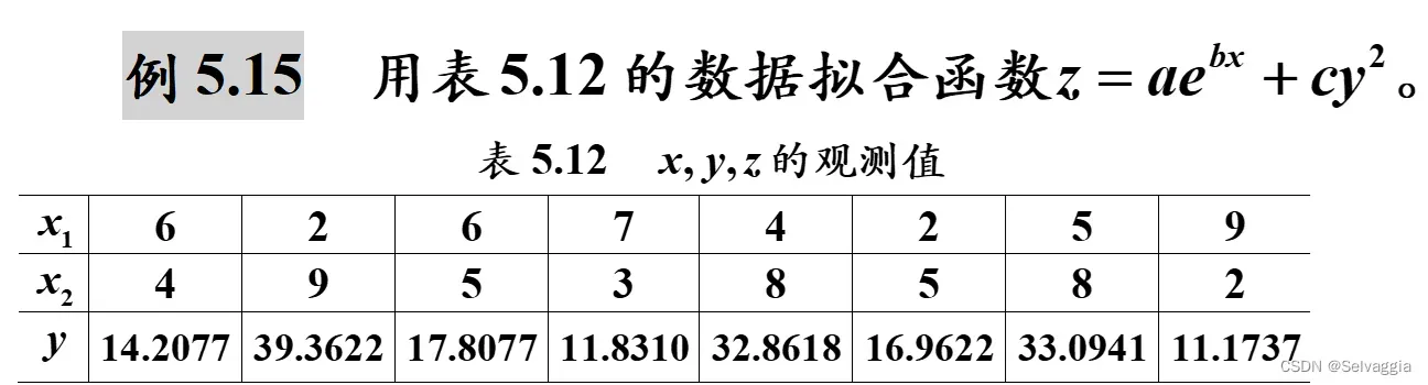
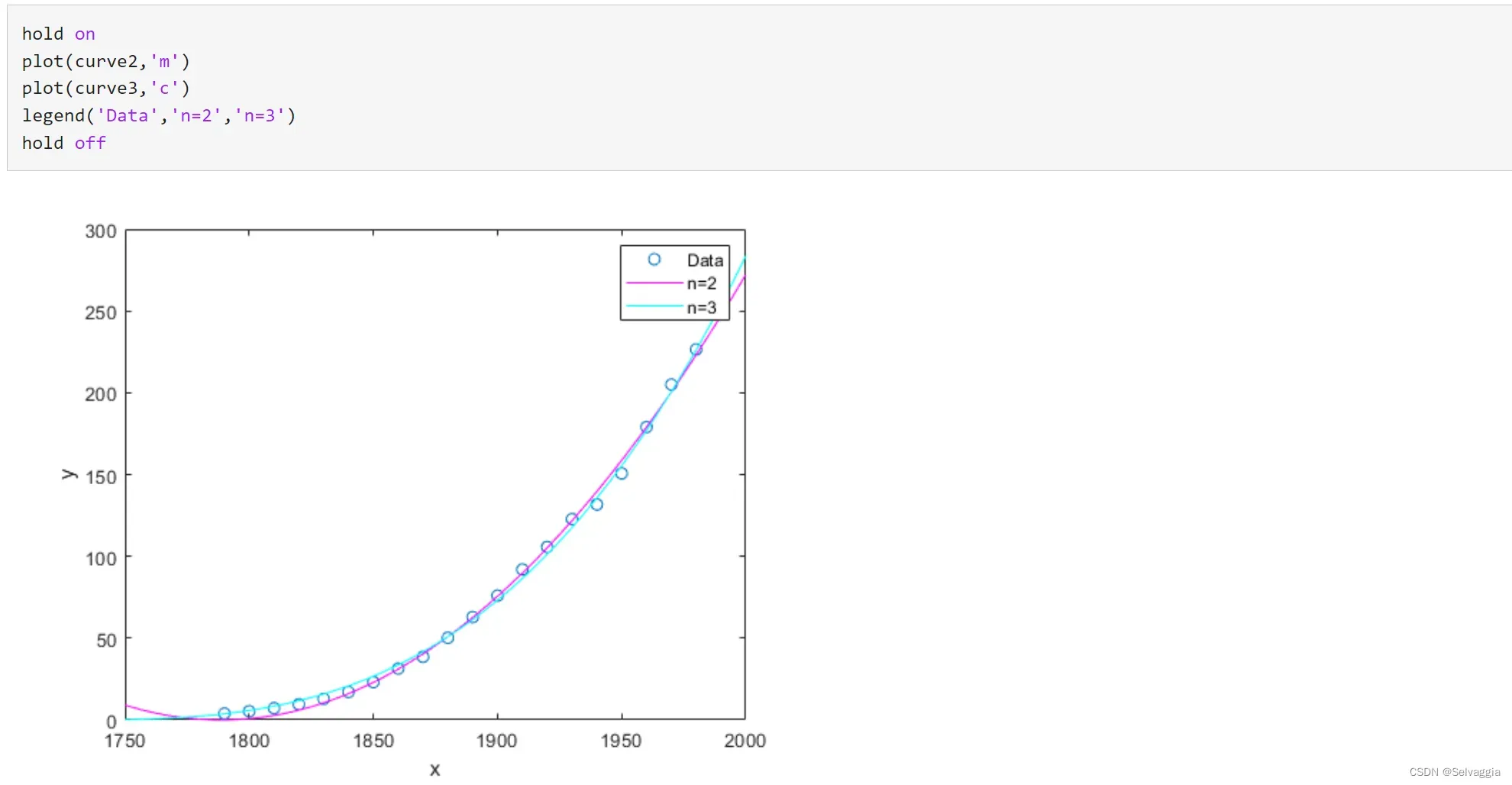
clc, clear, d=load('data5_15.txt');
xy0=d([1,2],:)'; z0=d(3,:)';
g=fittype('a*exp(b*x)+c*y^2','dependent','z','independent',{'x', 'y'})
[f,st]=fit(xy0,z0,g,'StartPoint',rand(1,3))
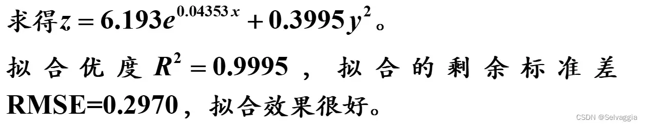
g =
     General model:
     g(a,b,c,x,y) = a*exp(b*x)+c*y^2

     General model:
     f(x,y) = a*exp(b*x)+c*y^2
     Coefficients (with 95% confidence bounds):
       a =       6.193  (5.043, 7.343)
       b =     0.04353  (0.01983, 0.06723)
       c =      0.3995  (0.3856, 0.4135)


st =
           sse: 0.4410
       rsquare: 0.9995
           dfe: 5
    adjrsquare: 0.9993
          rmse: 0.2970
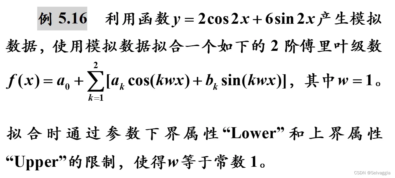
clc, clear
x0=[1:50]'; y0=2*cos(2*x0)+6*sin(2*x0);
lb=[-inf*ones(1,5),1]; ub=[inf*ones(1,5),1];
%要拟合的这个傅里叶函数有6个要拟合的参数
%w参数在最后一个位置,约束w=1
[f,g]=fit(x0,y0,'fourier2','Lower',lb,'Upper',ub)
f =
     General model Fourier2:
     f(x) =  a0 + a1*cos(x*w) + b1*sin(x*w) +
               a2*cos(2*x*w) + b2*sin(2*x*w)
     Coefficients (with 95% confidence bounds):
       a0 =    3.96e-17  (-3.85e-16, 4.642e-16)
       a1 =  -5.136e-16  (-1.115e-15, 8.836e-17)
       b1 =  -3.754e-17  (-6.366e-16, 5.615e-16)
       a2 =           2  (2, 2)
       b2 =           6  (6, 6)
       w =           1  (fixed at bound)

g =
           sse: 9.9988e-29
       rsquare: 1
           dfe: 45
    adjrsquare: 1
          rmse: 1.4906e-15

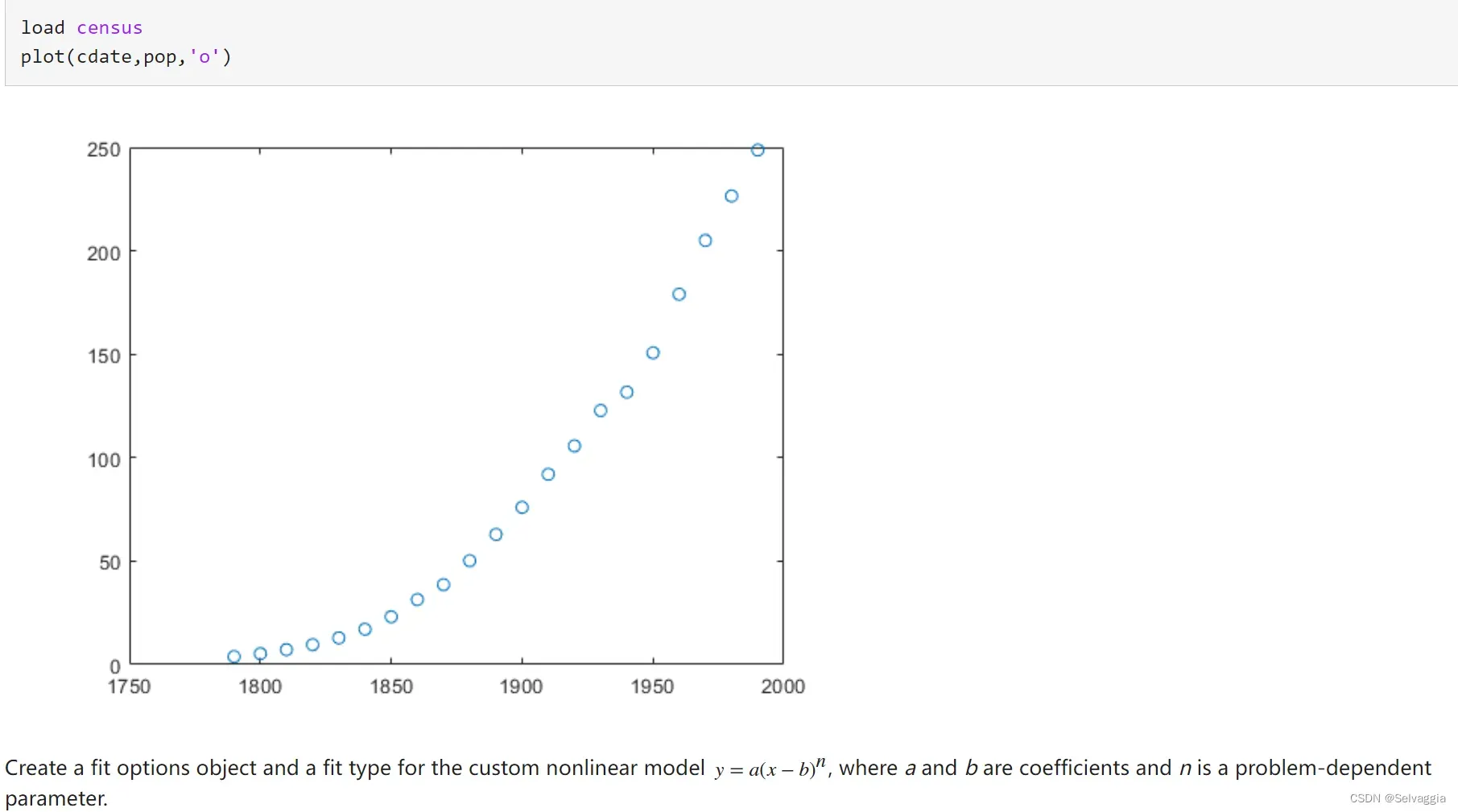
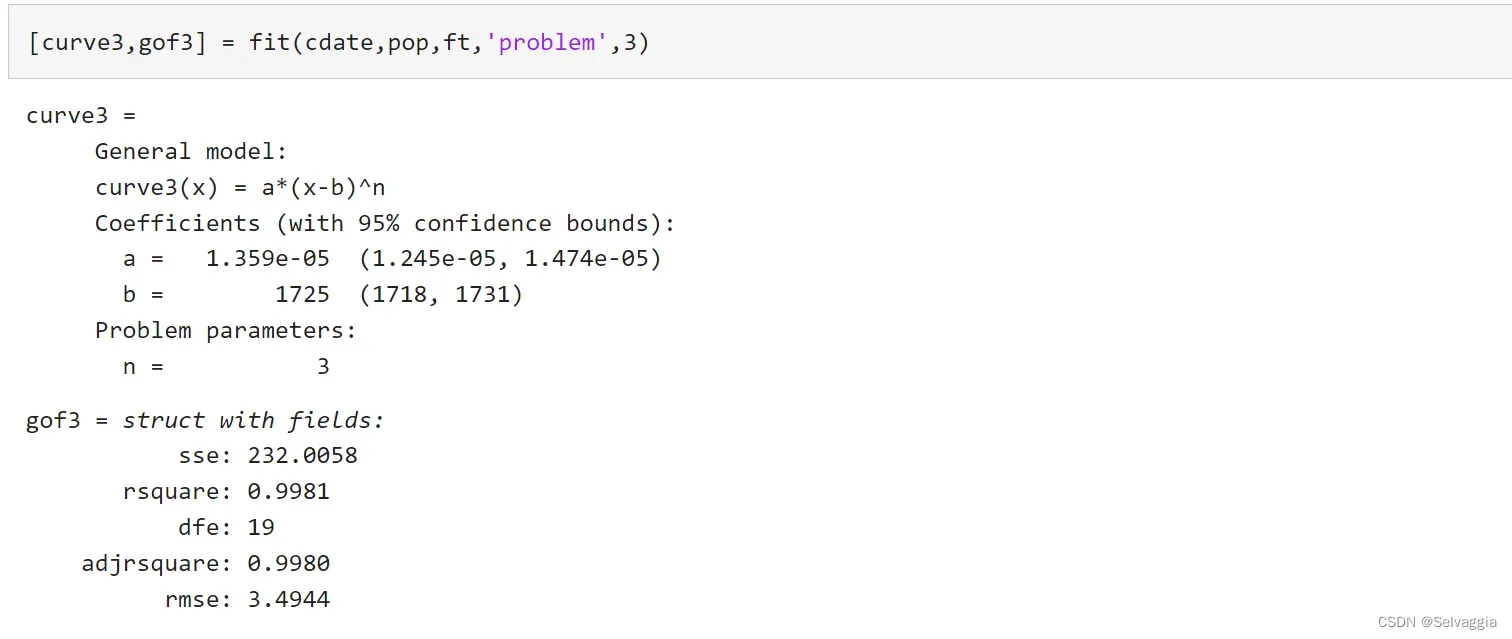
经典问题的拟合方式
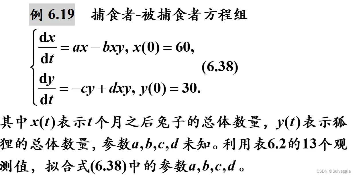
clc, clear
t0=[0	1	2	3	4	5	6	8	10	12	14	16	18]';
x0=[60	63	64	63	61	58	53	44	39	38	41	46	53]';
y0=[30	34	38	44	50	55	58	56	47	38	30	27	26]';
dt=diff(t0); dx=diff(x0); dy=diff(y0);
temp=x0(1:end-1).*y0(1:end-1);
mat=[x0(1:end-1), -temp,zeros(12,2)
    zeros(12,2), -y0(1:end-1), temp]; %构造线性方程组的系数矩阵
const=[dx./dt; dy./dt];  %构造线性方程组的常数项列
abcd=mat\const  %拟合参数a,b,c,d
文章出处登录后可见!