文章目录
前言
激活函数是一种特殊的非线性函数,它能够在神经网络中使用,其作用是将输入信号转化成输出信号。它将神经元中的输入信号转换为一个有意义的输出,从而使得神经网络能够学习和识别复杂的模式。常用的激活函数有 Sigmoid、ReLU、Leaky ReLU 和 ELU 等。大论文理论部分需要介绍激活函数,需要自己贴图,用python画图比matlab好很多,推荐,可以根据自己的需要对代码进行注释得到相应的激活函数曲线,暂时编写了三种论文常见的激活函数代码,后续会进行更新其他激活函数画图的代码。如果有帮助,请收藏关注一下我吧,如果有更多的需求欢迎私信我
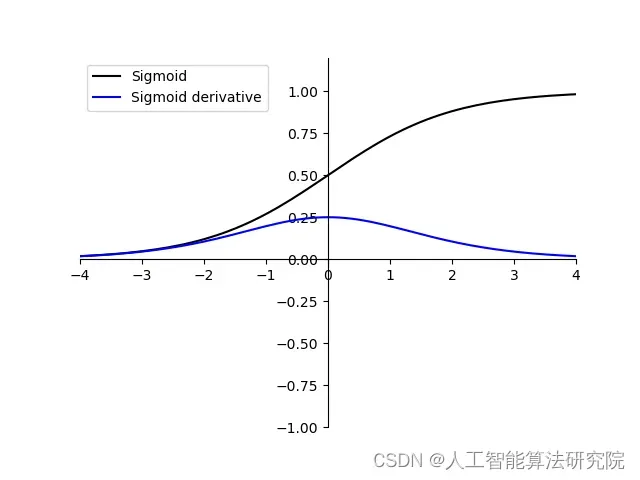
1. Sigmoid
sigmoid 是使用范围最广的一类激活函数,具有指数函数形状,它在物理意义上最为接近生物神经元,是一个在生物学中常见的S型的函数,也称为S型生长曲线。此外,(0, 1) 的输出还可以被表示作概率,或用于输入的归一化,代表性的如Sigmoid交叉熵损失函数。

		import math
import numpy as np
import matplotlib.pyplot as plt

# set x's range
x = np.arange(-10, 10, 0.1)
y1 = 1 / (1 + math.e ** (-x))  # sigmoid
# y11=math.e**(-x)/((1+math.e**(-x))**2)
y11 = 1 / (2 + math.e ** (-x)+ math.e ** (x))  # sigmoid的导数
y2 = (math.e ** (x) - math.e ** (-x)) / (math.e ** (x) + math.e ** (-x))  # tanh
y22 = 1-y2*y2  # tanh函数的导数
y3 = np.where(x < 0, 0, x)  # relu
y33 = np.where(x < 0, 0, 1)  # ReLU函数导数
plt.xlim(-4, 4)
plt.ylim(-1, 1.2)
ax = plt.gca()
ax.spines['right'].set_color('none')
ax.spines['top'].set_color('none')
ax.xaxis.set_ticks_position('bottom')
ax.yaxis.set_ticks_position('left')
ax.spines['bottom'].set_position(('data', 0))
ax.spines['left'].set_position(('data', 0))

# Draw pic
plt.plot(x, y1, label='Sigmoid', linestyle="-", color="black")
plt.plot(x, y11, label='Sigmoid derivative', linestyle="-", color="blue")
#plt.plot(x, y2, label='Tanh', linestyle="-", color="black")
#plt.plot(x, y22, label='Tanh derivative', linestyle="-", color="blue")
#plt.plot(x, y3, label='Tanh', linestyle="-", color="black")
#plt.plot(x, y33, label='Tanh derivative', linestyle="-", color="blue")
# Title
plt.legend(['Sigmoid', 'Tanh', 'Relu'])
plt.legend(['Sigmoid', 'Sigmoid derivative'])  # y1 y11
#plt.legend(['Tanh', 'Tanh derivative'])  # y2 y22
#plt.legend(['Relu', 'Relu derivative'])  # y3 y33

#plt.legend(['Sigmoid', 'Sigmoid derivative', 'Relu', 'Relu derivative', 'Tanh', 'Tanh derivative'])  # y3 y33
# plt.legend(loc='upper left')  # 将图例放在左上角

# save pic
# plt.savefig('plot_test.png', dpi=100)
plt.savefig(r"./")

# show it!!
plt.show()
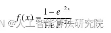
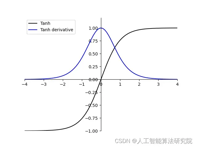
2. tanh
tanh在sigmoid基础上做出改进,与sigmoid相比,tanh输出均值为0,能够加快网络的收敛速度。然而,tanh同样存在梯度消失现象。
		import math
import numpy as np
import matplotlib.pyplot as plt

# set x's range
x = np.arange(-10, 10, 0.1)
y1 = 1 / (1 + math.e ** (-x))  # sigmoid
# y11=math.e**(-x)/((1+math.e**(-x))**2)
y11 = 1 / (2 + math.e ** (-x)+ math.e ** (x))  # sigmoid的导数
y2 = (math.e ** (x) - math.e ** (-x)) / (math.e ** (x) + math.e ** (-x))  # tanh
y22 = 1-y2*y2  # tanh函数的导数
y3 = np.where(x < 0, 0, x)  # relu
y33 = np.where(x < 0, 0, 1)  # ReLU函数导数
plt.xlim(-4, 4)
plt.ylim(-1, 1.2)
ax = plt.gca()
ax.spines['right'].set_color('none')
ax.spines['top'].set_color('none')
ax.xaxis.set_ticks_position('bottom')
ax.yaxis.set_ticks_position('left')
ax.spines['bottom'].set_position(('data', 0))
ax.spines['left'].set_position(('data', 0))

# Draw pic
#plt.plot(x, y1, label='Sigmoid', linestyle="-", color="black")
#plt.plot(x, y11, label='Sigmoid derivative', linestyle="-", color="blue")

#plt.plot(x, y2, label='Tanh', linestyle="-", color="black")
#plt.plot(x, y22, label='Tanh derivative', linestyle="-", color="blue")

plt.plot(x, y3, label='Tanh', linestyle="-", color="black")
plt.plot(x, y33, label='Tanh derivative', linestyle="-", color="blue")

# Title
plt.legend(['Sigmoid', 'Tanh', 'Relu'])
#plt.legend(['Sigmoid', 'Sigmoid derivative'])  # y1 y11
#plt.legend(['Tanh', 'Tanh derivative'])  # y2 y22
plt.legend(['Relu', 'Relu derivative'])  # y3 y33

#plt.legend(['Sigmoid', 'Sigmoid derivative', 'Relu', 'Relu derivative', 'Tanh', 'Tanh derivative'])  # y3 y33
# plt.legend(loc='upper left')  # 将图例放在左上角

# save pic
# plt.savefig('plot_test.png', dpi=100)
plt.savefig(r"./")

# show it!!
plt.show()
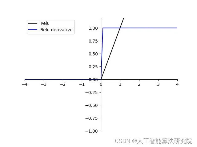
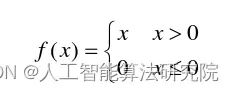
3. ReLU
ReLU是针对sigmoid与tanh中存在的梯度消失问题提出的激活活函数。由于ReLU在x大于0时梯度保持不变,从而解决了tanh中存在的梯度消失现象。但是,在训练过程中,当x进入到小于0的范围时,激活函数输出一直为0,使得网络无法更新权重,出现了“神经元死亡”现象。同时,与sigmoid相似,ReLU输出均值大于0,同样存在偏移现象。
		import math
import numpy as np
import matplotlib.pyplot as plt

# set x's range
x = np.arange(-10, 10, 0.1)
y1 = 1 / (1 + math.e ** (-x))  # sigmoid
# y11=math.e**(-x)/((1+math.e**(-x))**2)
y11 = 1 / (2 + math.e ** (-x)+ math.e ** (x))  # sigmoid的导数
y2 = (math.e ** (x) - math.e ** (-x)) / (math.e ** (x) + math.e ** (-x))  # tanh
y22 = 1-y2*y2  # tanh函数的导数
y3 = np.where(x < 0, 0, x)  # relu
y33 = np.where(x < 0, 0, 1)  # ReLU函数导数
plt.xlim(-4, 4)
plt.ylim(-1, 1.2)
ax = plt.gca()
ax.spines['right'].set_color('none')
ax.spines['top'].set_color('none')
ax.xaxis.set_ticks_position('bottom')
ax.yaxis.set_ticks_position('left')
ax.spines['bottom'].set_position(('data', 0))
ax.spines['left'].set_position(('data', 0))

# Draw pic
#plt.plot(x, y1, label='Sigmoid', linestyle="-", color="black")
#plt.plot(x, y11, label='Sigmoid derivative', linestyle="-", color="blue")

#plt.plot(x, y2, label='Tanh', linestyle="-", color="black")
#plt.plot(x, y22, label='Tanh derivative', linestyle="-", color="blue")

plt.plot(x, y3, label='Tanh', linestyle="-", color="black")
plt.plot(x, y33, label='Tanh derivative', linestyle="-", color="blue")


# Title
plt.legend(['Sigmoid', 'Tanh', 'Relu'])
#plt.legend(['Sigmoid', 'Sigmoid derivative'])  # y1 y11
#plt.legend(['Tanh', 'Tanh derivative'])  # y2 y22
plt.legend(['Relu', 'Relu derivative'])  # y3 y33

#plt.legend(['Sigmoid', 'Sigmoid derivative', 'Relu', 'Relu derivative', 'Tanh', 'Tanh derivative'])  # y3 y33
# plt.legend(loc='upper left')  # 将图例放在左上角

# save pic
# plt.savefig('plot_test.png', dpi=100)
plt.savefig(r"./")

# show it!!
plt.show()
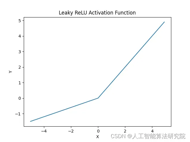
4. Leaky ReLU
Leaky ReLU 通过把 x 的非常小的线性分量给予负输入(0.01x)来调整负值的零梯度(zero gradients)问题;
leak 有助于扩大 ReLU 函数的范围,通常 a 的值为 0.01 左右;
Leaky ReLU 的函数范围是(负无穷到正无穷)。
注意:从理论上讲,Leaky ReLU 具有 ReLU 的所有优点,而且 Dead ReLU 不会有任何问题,但在实际操作中,尚未完全证明 Leaky ReLU 总是比 ReLU 更好。
import numpy as np
import matplotlib.pyplot as plt

# Generate data points
x = np.arange(-5, 5, 0.1)

# Compute Leaky ReLU for different values of alpha
alpha = 0.3 # alpha is the slope of the negative part
y_leaky_relu = np.maximum(x, x * alpha)

# Plotting the Leaky ReLU graph
plt.plot(x, y_leaky_relu)
plt.title("Leaky ReLU Activation Function")
plt.xlabel("X")
plt.ylabel("Y")

 # Show the plot
 plt.show()
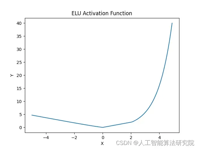
5. ELU
ELU(Exponential Linear Unit)激活函数是一种添加了指数项的非线性激活函数,它的表达式如下:
ELU(x) = {x, x > 0; α(e^x-1), x <= 0}
其中α是一个超参数。ELU 激活函数的特征在于输入为负时会有正值的输出,而不是 0。这样可以有效地避免神经元死亡问题。 ELU 激活函数有助于神经元学习复杂的非线性函数,可以帮助神经元学习复杂的非线性特征。
import numpy as np
import matplotlib.pyplot as plt

# Generate data points
x = np.arange(-5, 5, 0.1)

# Compute ELU for different values of alpha and lambda
alpha = 0.3  # alpha is the slope of the negative part
lamda = 1  # lambda is the magnitude of the negative part
y_elu = np.maximum(x, alpha * (np.exp(x) - 1)) + lamda * (np.maximum(0, x) - x)  # Compute ELU

# Plotting the ELU graph
plt.plot(x, y_elu)
plt.title("ELU Activation Function")
plt.xlabel("X")
plt.ylabel("Y")

# Show the plot
plt.show()
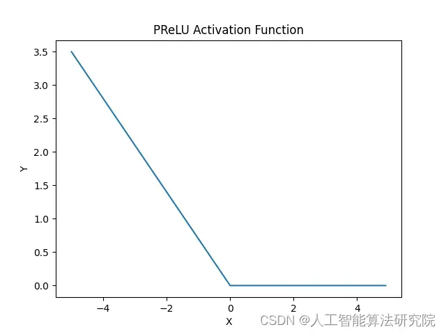
6.PReLU
PReLU 激活函数是一种可训练的改进版本的 Leaky ReLU 激活函数,它使用了可训练的斜率 α 作为超参数。PReLU 的定义如下:
f(x) = max(αx, x)
其中α是可学习的斜率,通常初始化为 0.25 或者 0.01。PReLU 和 Leaky ReLU 很相似,但 PReLU 能够根据输入和预期而学习一个最佳的斜率 α。这能够避免使用常量 α 时所带来的问题。
import numpy as np
import matplotlib.pyplot as plt

# Generate data points
x = np.arange(-5, 5, 0.1)

# Compute PReLU for different values of alpha and lambda
alpha = 0.3 # alpha is the slope of the negative part
lamda = 1 # lambda is the magnitude of the negative part

 y_prelu = lamda * (np.maximum(0, x) - x) + alpha * np.minimum(0, x) # Compute PReLU

    # Plotting the PReLU graph
plt.plot(x, y_prelu)
plt.title("PReLU Activation Function")
plt.xlabel("X")
plt.ylabel("Y")

 # Show the plot
 plt.show()
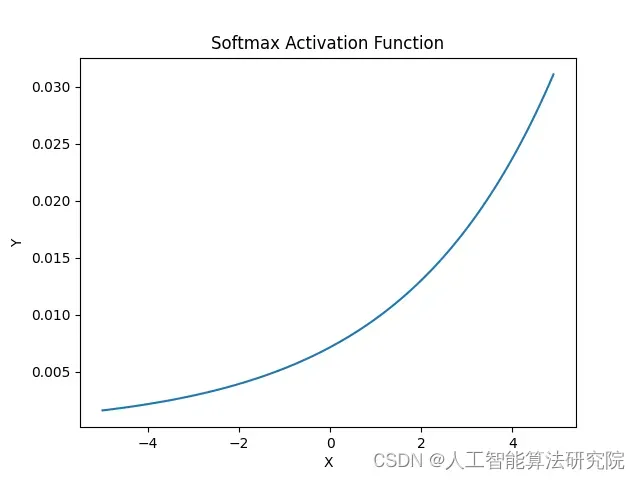
7. Softmax
Softmax 激活函数用于多分类问题,它在神经网络的最后一层被使用。Softmax 函数能够将输入信号转换为 0 到 1 之间的值,表示不同分类的可能性。Softmax 激活函数的定义如下:
Sj(z) = exp(zj) / Σk=1n exp(zk)
其中 zj 表示神经元的输入,n 表示神经元的个数,Sj(z) 表示神经元 j 的输出。Softmax 函数会将所有输出值相加为 1,并将每个输出值归一化到 0 到 1 之间。
import numpy as np
import matplotlib.pyplot as plt

# Generate data points
x = np.arange(-5, 5, 0.1)

# Compute Softmax for different values of beta and gamma
beta = 0.3 # beta is the slope of the negative part
gamma = 1 # gamma is the magnitude of the negative part

 y_softmax = gamma * (np.exp(beta*x) / np.sum(np.exp(beta*x))) # Compute Softmax

    # Plotting the Softmax graph
plt.plot(x, y_softmax)
plt.title("Softmax Activation Function")
plt.xlabel("X")
plt.ylabel("Y")

 # Show the plot
 plt.show()
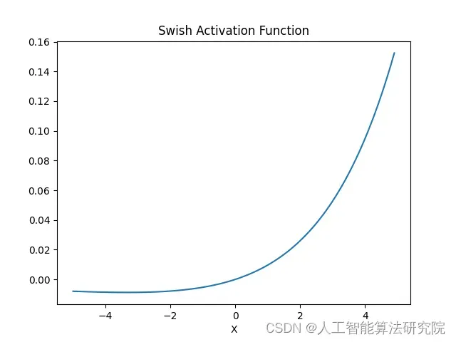
8. Swish
Swish 激活函数是一种新型的激活函数,它的表达式如下:
S(x) = x * Sigmoid(x)
其中 Sigmoid 函数为双曲正切函数,它的定义如下:
Sigmoid(x) = 1 / (1 + exp(-x))
Swish 函数可以将输入信号转化为 0 到 1 之间的值,表示不同分类的可能性。特别是,在神经网络中,Swish 激活函数可以帮助神经元学习复杂的非线性函数。
import numpy as np
import matplotlib.pyplot as plt

# Generate data points
x = np.arange(-5, 5, 0.1)

 # Compute Swish for different values of beta and gamma
beta = 0.3 # beta is the slope of the negative part
gamma = 1 # gamma is the magnitude of the negative part

 y_swish = gamma * x * (np.exp(beta*x) / np.sum(np.exp(beta*x))) # Compute Softmax

    # Plotting the Swish graph
plt.plot(x, y_swish)
plt.title("Swish Activation Function")
plt.xlabel("X")
plt
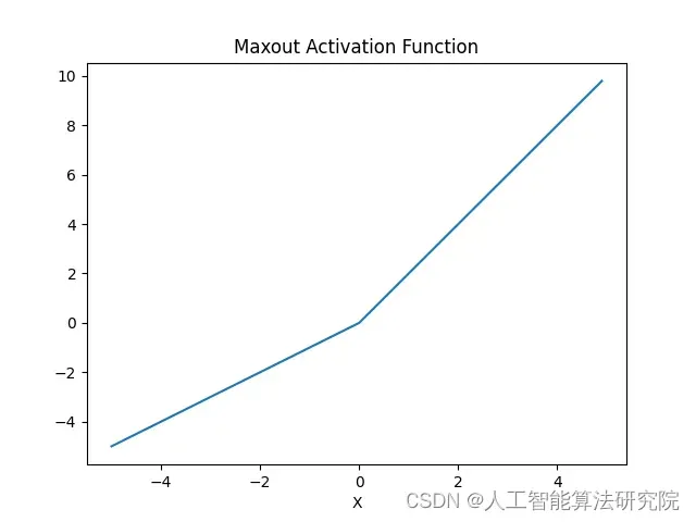
9. Maxout
Maxout 激活函数是一种新型的激活函数,它可以用来代替传统的 ReLU 和 Sigmoid 函数。Maxout 激活函数的表达式如下:
Maxout(x) = MAX{ f1(x), f2(x) }
其中 f1 和 f2 是 Maxout 的两个参数,它们分别对应于 Maxout 的两个输入。Maxout 的最大值就是它的输出值。Maxout 激活函数可以帮助神经元学习复杂的非线性函数,特别是在神经网络中。
import numpy as np
import matplotlib.pyplot as plt

# Generate data points
x = np.arange(-5, 5, 0.1)

 # Compute Maxout for different values of alpha and beta
alpha = 1 # alpha is the slope of the linear part
beta = 2 # beta is the slope of the non-linear part

y_maxout = np.maximum(alpha*x, beta*x) # Compute Maxout

    # Plotting the Maxout graph
plt.plot(x, y_maxout)
plt.title("Maxout Activation Function")
plt.xlabel("X")
plt.show()
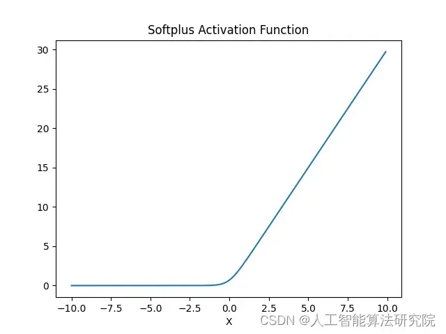
10. Softplus
Softplus 激活函数是一种渐进型的非线性激活函数,它的表达式如下:
Softplus(x) = ln (1 + e^x)
Softplus 激活函数在输入为 0 时取值为 0,它的输出随着输入增大而变大,但不会到负无穷大。Softplus 激活函数有助于神经元学习复杂的非线性函数,可以帮助神经元学习复杂的非线性特征。
import numpy as np
import matplotlib.pyplot as plt

# Generate data points
x = np.arange(-10, 10, 0.1)

 # Compute Softplus for different values of alpha and beta
alpha = 1 # alpha is the slope of the linear part
beta = 2 # beta is the slope of the non-linear part

y_softplus = np.log(1 + np.exp(alpha*x + beta*x)) # Compute Softplus

    # Plotting the Softplus graph
plt.plot(x, y_softplus)
plt.title("Softplus Activation Function")
plt.xlabel("X")
plt.show()
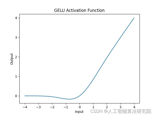
11. GELU
GELU 激活函数是一种基于 Gaussian 概率分布的非线性函数,它可以将输入信号转换为大于 0 的值或小于 0 的值。GELU 激活函数的特点是,它的梯度随输入的大小而变化,这使得它能够有效地学习复杂的非线性问题。此外,GELU 激活函数还具有快速优化和泛化性能优异的优势。
import numpy as np
import matplotlib.pyplot as plt


def gelu(x):
    return 0.5 * x * (1 + np.tanh(np.sqrt(2 / np.pi) * (x + 0.044715 * np.power(x, 3))))


# Generate values for x axis
x_axis = np.arange(-4, 4, 0.01)
# Calculate corresponding y axis values using gelu() function
y_axis = [gelu(i) for i in x_axis]
# Plot the points
plt.plot(x_axis, y_axis)
# Set the x and y axes labels and title of the graph
plt.title("GELU Activation Function")
plt.xlabel('Input')
plt.ylabel('Output')

# Display the graph
plt.show()
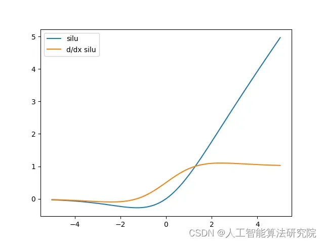
12. SILU
SiLU激活函数(又称Sigmoid-weighted Linear Unit)是一种新型的非线性激活函数,它将sigmoid函数和线性单元相结合,以此来获得在低数值区域中表现良好的非线性映射能力。SiLU激活函数的特征是它在低数值区域中表现较为平滑,而在高数值区域中表现起来十分“锐利”,从而能够有效地避免过度学习的问题。
import matplotlib.pyplot as plt
import numpy as np
from scipy.special import expit


# 定义SiLU函数和导函数
def silu(x):
    return x * expit(x)


def dsilu(x):
    return expit(x) * (1 + x * (1 - expit(x)))

    # 生成-5到5之间的100个数据点   计算SiLU和导SiLU函数的值   绘图显示 SiLU 函数以及导函数的曲线


x = np.linspace(-5, 5, 100)  # 生成-5到5之间的100个数据点

y = silu(x)  # 计算sigmoid函数的值
y_prime = dsilu(x) #计算sigmoid 导函数的值

plt.plot(x, y, label="silu")  # 绘图 显示 SiLU 函数以及导函数的曲线。
plt.plot(x, y_prime, label="d/dx silu")
plt.legend()
plt.show()
总结
本文介绍Sigmoid,ReLU,Tanh这三种常见的激活函数及利用python画图代码,后续会持续更新,有帮助也请免费点个小小的收藏吧,有更多的需求帮助可关注私信我。关注即免费获取大量人工智能学习资料。
文章出处登录后可见!