多模态模型学习1——CLIP对比学习 语言-图像预训练模型
- 学习前言
- 什么是CLIP模型
- 代码下载
- CLIP实现思路
- 一、网络结构介绍
- 1、Image Encoder
- a、Patch+Position Embedding
- b、Transformer Encoder
- I、Self-attention结构解析
- II、Self-attention的矩阵运算
- III、MultiHead多头注意力机制
- IV、TransformerBlock的构建。
- c、整个VIT模型的构建
- 2、Text Encoder
- 二、训练部分
- 训练自己的CLIP模型
- 一、数据集的准备
- 二、数据集的格式
- 三、开始网络训练
- 四、训练结果预测
学习前言
学了一些多模态的知识,CLIP算是其中最重要也是最通用的一环,一起来看一下吧。

什么是CLIP模型
CLIP的全称是Contrastive Language-Image Pre-Training,中文是对比语言-图像预训练,是一个预训练模型,简称为CLIP。
该模型是 OpenAI 在 2021 年发布的,最初用于匹配图像和文本的预训练神经网络模型,这个任务在多模态领域比较常见,可以用于文本图像检索,CLIP是近年来在多模态研究领域的经典之作。该模型大量的成对互联网数据进行预训练,在很多任务表现上达到了目前最佳表现(SOTA) 。
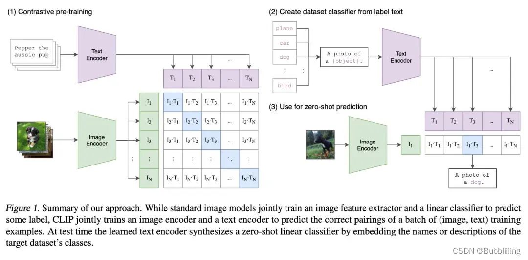
CLIP的思想非常简单,只需要看懂这幅图就可以了,左边是训练的原理,CLIP一共有两个模态,一个是文本模态,一个是视觉模态,分别对应了Text Encoder和Image Encoder。
Text Encoder用于对文本进行编码,获得其Embedding;
Image Encoder用于对图片编码,获得其Embedding。
两个Embedding均为一定长度的单一向量。
在训练时,假设一个批次中有64个文本图像对,此时我们会同时获得64个图片和64个文本,首先我们从64个文本图像对中取出一个文本图像对,成对的文本图像对是天然的正样本,它们是配对的。
而对于这个样本的文本来讲,其它63个图像都为负样本,它们是不配对的。
而对于这个样本的图像来讲,其它63个文本都为负样本,它们是不配对的。
在这个批次中,64个文本图像对,可以获得的图像embedding和文本embedding为:
visual_embedding 	[64, embedding_size]
text_embedding		[64, embedding_size]
visual_embedding的第x行和text_embedding的第x行是成对的。
我们使用visual_embedding 叉乘 text_embedding,得到一个[64, 64]的矩阵,那么对角线上的值便是成对特征内积得到的,如果visual_embedding和对应的text_embedding越相似,那么它的值便越大。
我们选取[64, 64]矩阵中的第一行,代表第1个图片与64个文本的相似程度,其中第1个文本是正样本,我们将这一行的标签设置为1,那么我们就可以使用交叉熵进行训练,尽量把第1个图片和第一个文本的内积变得更大,那么它们就越相似。
每一行都做同样的工作,那么[64, 64]的矩阵,它的标签就是[1,2,3,4,5,6……,64],在计算机中,标签从0开始,所以实际标签为[0,1,2,3,4,5……,63]。
代码下载
Github源码下载地址为:
https://github.com/bubbliiiing/clip-pytorch
复制该路径到地址栏跳转。
CLIP实现思路
一、网络结构介绍
1、Image Encoder
a、Patch+Position Embedding
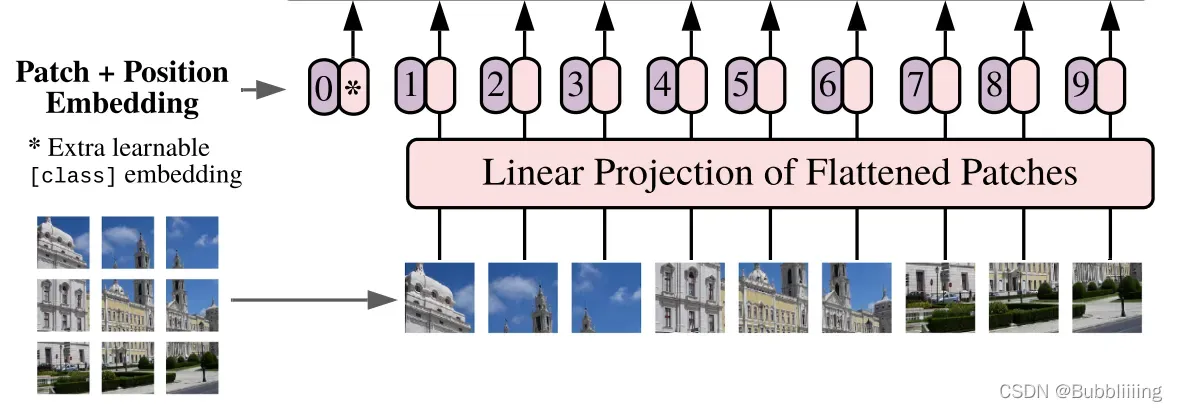
Patch+Position Embedding的作用主要是对输入进来的图片进行分块处理,每隔一定的区域大小划分图片块。然后将划分后的图片块组合成序列。
该部分首先对输入进来的图片进行分块处理,处理方式其实很简单,使用的是现成的卷积。由于卷积使用的是滑动窗口的思想,我们只需要设定特定的步长,就可以输入进来的图片进行分块处理了。
在VIT中,我们常设置这个卷积的卷积核大小为16×16,步长也为16×16,此时卷积就会每隔16个像素点进行一次特征提取,由于卷积核大小为16×16,两个图片区域的特征提取过程就不会有重叠。当我们输入的图片是224, 224, 3的时候,我们可以获得一个14, 14, 768的特征层。

下一步就是将这个特征层组合成序列,组合的方式非常简单,就是将高宽维度进行平铺,14, 14, 768在高宽维度平铺后,获得一个196, 768的特征层。平铺完成后,我们会在图片序列中添加上Cls Token,该Token会作为一个单位的序列信息一起进行特征提取,图中的这个0*就是Cls Token,我们此时获得一个197, 768的特征层。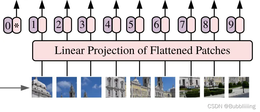
添加完成Cls Token后,再为所有特征添加上位置信息,这样网络才有区分不同区域的能力。添加方式其实也非常简单,我们生成一个197, 768的参数矩阵,这个参数矩阵是可训练的,把这个矩阵加上197, 768的特征层即可。
到这里,Patch+Position Embedding就构建完成了,构建代码如下:
class VisionTransformer(nn.Module):
    def __init__(self, input_resolution: int, patch_size: int, width: int, layers: int, heads: int, output_dim: int):
        super().__init__()
        self.input_resolution = input_resolution
        self.output_dim = output_dim
        #-----------------------------------------------#
        #   224, 224, 3 -> 196, 768
        #-----------------------------------------------#
        self.conv1 = nn.Conv2d(in_channels=3, out_channels=width, kernel_size=patch_size, stride=patch_size, bias=False)

        scale = width ** -0.5
        #--------------------------------------------------------------------------------------------------------------------#
        #   class_embedding部分是transformer的分类特征。用于堆叠到序列化后的图片特征中,作为一个单位的序列特征进行特征提取。
        #
        #   在利用步长为16x16的卷积将输入图片划分成14x14的部分后,将14x14部分的特征平铺,一幅图片会存在序列长度为196的特征。
        #   此时生成一个class_embedding,将class_embedding堆叠到序列长度为196的特征上,获得一个序列长度为197的特征。
        #   在特征提取的过程中,class_embedding会与图片特征进行特征的交互。最终分类时,我们取出class_embedding的特征,利用全连接分类。
        #--------------------------------------------------------------------------------------------------------------------#
        #   196, 768 -> 197, 768
        self.class_embedding = nn.Parameter(scale * torch.randn(width))
        #--------------------------------------------------------------------------------------------------------------------#
        #   为网络提取到的特征添加上位置信息。
        #   以输入图片为224, 224, 3为例,我们获得的序列化后的图片特征为196, 768。加上class_embedding后就是197, 768
        #   此时生成的pos_Embedding的shape也为197, 768,代表每一个特征的位置信息。
        #--------------------------------------------------------------------------------------------------------------------#
        #   197, 768 -> 197, 768
        self.positional_embedding = nn.Parameter(scale * torch.randn((input_resolution // patch_size) ** 2 + 1, width))

    def forward(self, x: torch.Tensor):
        x = self.conv1(x)  # shape = [*, width, grid, grid]
        x = x.reshape(x.shape[0], x.shape[1], -1)  # shape = [*, width, grid ** 2]
        x = x.permute(0, 2, 1)  # shape = [*, grid ** 2, width]
        x = torch.cat([self.class_embedding.to(x.dtype) + torch.zeros(x.shape[0], 1, x.shape[-1], dtype=x.dtype, device=x.device), x], dim=1)  # shape = [*, grid ** 2 + 1, width]
        x = x + self.positional_embedding.to(x.dtype)
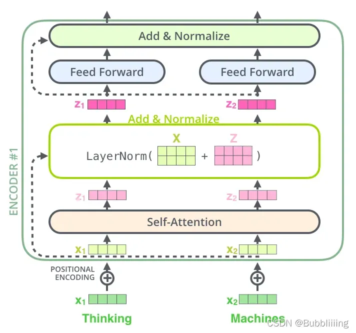
b、Transformer Encoder
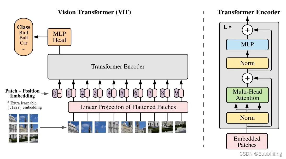
在上一步获得shape为197, 768的序列信息后,将序列信息传入Transformer Encoder进行特征提取,这是Transformer特有的Multi-head Self-attention结构,通过自注意力机制,关注每个图片块的重要程度。
I、Self-attention结构解析
看懂Self-attention结构,其实看懂下面这个动图就可以了,动图中存在一个序列的三个单位输入,每一个序列单位的输入都可以通过三个处理(比如全连接)获得Query、Key、Value,Query是查询向量、Key是键向量、Value值向量。

如果我们想要获得input-1的输出,那么我们进行如下几步:
1、利用input-1的查询向量,分别乘上input-1、input-2、input-3的键向量,此时我们获得了三个score。
2、然后对这三个score取softmax,获得了input-1、input-2、input-3各自的重要程度。
3、然后将这个重要程度乘上input-1、input-2、input-3的值向量,求和。
4、此时我们获得了input-1的输出。
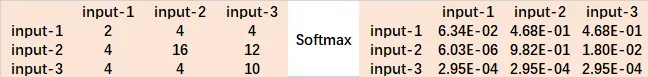
如图所示,我们进行如下几步:
1、input-1的查询向量为[1, 0, 2],分别乘上input-1、input-2、input-3的键向量,获得三个score为2,4,4。
2、然后对这三个score取softmax,获得了input-1、input-2、input-3各自的重要程度,获得三个重要程度为0.0,0.5,0.5。
3、然后将这个重要程度乘上input-1、input-2、input-3的值向量,求和,即
。
4、此时我们获得了input-1的输出 [2.0, 7.0, 1.5]。
上述的例子中,序列长度仅为3,每个单位序列的特征长度仅为3,在VIT的Transformer Encoder中,序列长度为197,每个单位序列的特征长度为768 // num_heads。但计算过程是一样的。在实际运算时,我们采用矩阵进行运算。
II、Self-attention的矩阵运算
实际的矩阵运算过程如下图所示。我以实际矩阵为例子给大家解析:
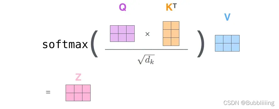
输出的每一行,都代表input-1、input-2、input-3,对当前input的贡献,我们对这个贡献值取一个softmax。

然后利用 score 叉乘 value,这一步可以通俗的理解为,将序列每个部分的重要程度重新施加到序列的值上去。

这个矩阵运算的代码如下所示,各位同学可以自己试试。
import numpy as np

def soft_max(z):
    t = np.exp(z)
    a = np.exp(z) / np.expand_dims(np.sum(t, axis=1), 1)
    return a

Query = np.array([
    [1,0,2],
    [2,2,2],
    [2,1,3]
])

Key = np.array([
    [0,1,1],
    [4,4,0],
    [2,3,1]
])

Value = np.array([
    [1,2,3],
    [2,8,0],
    [2,6,3]
])

scores = Query @ Key.T
print(scores)
scores = soft_max(scores)
print(scores)
out = scores @ Value
print(out)
III、MultiHead多头注意力机制
多头注意力机制的示意图如图所示:
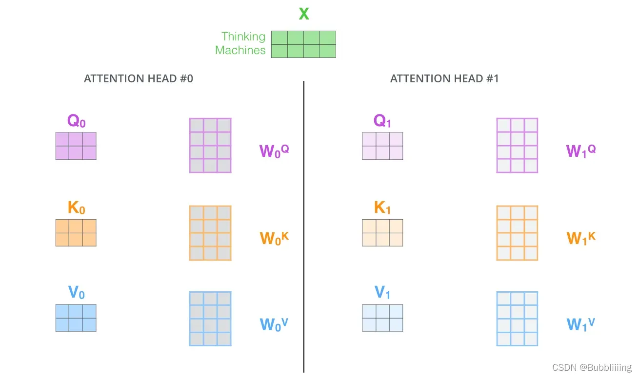
这幅图给人的感觉略显迷茫,我们跳脱出这个图,直接从矩阵的shape入手会清晰很多。
在第一步进行图像的分割后,我们获得的特征层为197, 768。
在施加多头的时候,我们直接对196, 768的最后一维度进行分割,比如我们想分割成12个头,那么矩阵的shepe就变成了196, 12, 64。
然后我们将196, 12, 64进行转置,将12放到前面去,获得的特征层为12, 196, 64。之后我们忽略这个12,把它和batch维度同等对待,只对196, 64进行处理,其实也就是上面的注意力机制的过程了。
下面这个代码并未在CLIP中使用,CLIP直接使用了nn.MultiheadAttention模块计算多头注意力,下面这个代码是其他部分的Vision Transformer截取过来的,方便各位理解。
#--------------------------------------------------------------------------------------------------------------------#
#   Attention机制
#   将输入的特征qkv特征进行划分,首先生成query, key, value。query是查询向量、key是键向量、v是值向量。
#   然后利用 查询向量query 叉乘 转置后的键向量key,这一步可以通俗的理解为,利用查询向量去查询序列的特征,获得序列每个部分的重要程度score。
#   然后利用 score 叉乘 value,这一步可以通俗的理解为,将序列每个部分的重要程度重新施加到序列的值上去。
#--------------------------------------------------------------------------------------------------------------------#
class Attention(nn.Module):
    def __init__(self, dim, num_heads=8, qkv_bias=False, attn_drop=0., proj_drop=0.):
        super().__init__()
        self.num_heads  = num_heads
        self.scale      = (dim // num_heads) ** -0.5

        self.qkv        = nn.Linear(dim, dim * 3, bias=qkv_bias)
        self.attn_drop  = nn.Dropout(attn_drop)
        self.proj       = nn.Linear(dim, dim)
        self.proj_drop  = nn.Dropout(proj_drop)

    def forward(self, x):
        B, N, C     = x.shape
        qkv         = self.qkv(x).reshape(B, N, 3, self.num_heads, C // self.num_heads).permute(2, 0, 3, 1, 4)
        q, k, v     = qkv[0], qkv[1], qkv[2]

        attn = (q @ k.transpose(-2, -1)) * self.scale
        attn = attn.softmax(dim=-1)
        attn = self.attn_drop(attn)

        x = (attn @ v).transpose(1, 2).reshape(B, N, C)
        x = self.proj(x)
        x = self.proj_drop(x)
        return x
IV、TransformerBlock的构建。
在完成MultiHeadSelfAttention的构建后,我们需要在其后加上两个全连接。就构建了整个TransformerBlock。
class ResidualAttentionBlock(nn.Module):
    def __init__(self, d_model: int, n_head: int, attn_mask: torch.Tensor = None):
        super().__init__()

        self.attn = nn.MultiheadAttention(d_model, n_head)
        self.ln_1 = LayerNorm(d_model)
        self.mlp = nn.Sequential(OrderedDict([
            ("c_fc", nn.Linear(d_model, d_model * 4)),
            ("gelu", QuickGELU()),
            ("c_proj", nn.Linear(d_model * 4, d_model))
        ]))
        self.ln_2 = LayerNorm(d_model)
        self.attn_mask = attn_mask

    def attention(self, x: torch.Tensor):
        self.attn_mask = self.attn_mask.to(dtype=x.dtype, device=x.device) if self.attn_mask is not None else None
        return self.attn(x, x, x, need_weights=False, attn_mask=self.attn_mask)[0]

    def forward(self, x: torch.Tensor):
        x = x + self.attention(self.ln_1(x))
        x = x + self.mlp(self.ln_2(x))
        return x
c、整个VIT模型的构建
整个VIT模型由一个Patch+Position Embedding加上多个TransformerBlock组成。典型的TransforerBlock的数量为12个。
from collections import OrderedDict

import torch
from torch import nn


class LayerNorm(nn.LayerNorm):
    """Subclass torch's LayerNorm to handle fp16."""

    def forward(self, x: torch.Tensor):
        orig_type = x.dtype
        ret = super().forward(x.type(torch.float32))
        return ret.type(orig_type)


class QuickGELU(nn.Module):
    def forward(self, x: torch.Tensor):
        return x * torch.sigmoid(1.702 * x)


class ResidualAttentionBlock(nn.Module):
    def __init__(self, d_model: int, n_head: int, attn_mask: torch.Tensor = None):
        super().__init__()

        self.attn = nn.MultiheadAttention(d_model, n_head)
        self.ln_1 = LayerNorm(d_model)
        self.mlp = nn.Sequential(OrderedDict([
            ("c_fc", nn.Linear(d_model, d_model * 4)),
            ("gelu", QuickGELU()),
            ("c_proj", nn.Linear(d_model * 4, d_model))
        ]))
        self.ln_2 = LayerNorm(d_model)
        self.attn_mask = attn_mask

    def attention(self, x: torch.Tensor):
        self.attn_mask = self.attn_mask.to(dtype=x.dtype, device=x.device) if self.attn_mask is not None else None
        return self.attn(x, x, x, need_weights=False, attn_mask=self.attn_mask)[0]

    def forward(self, x: torch.Tensor):
        x = x + self.attention(self.ln_1(x))
        x = x + self.mlp(self.ln_2(x))
        return x


class Transformer(nn.Module):
    def __init__(self, width: int, layers: int, heads: int, attn_mask: torch.Tensor = None):
        super().__init__()
        self.width = width
        self.layers = layers
        self.resblocks = nn.Sequential(*[ResidualAttentionBlock(width, heads, attn_mask) for _ in range(layers)])

    def forward(self, x: torch.Tensor):
        return self.resblocks(x)


class VisionTransformer(nn.Module):
    def __init__(self, input_resolution: int, patch_size: int, width: int, layers: int, heads: int, output_dim: int):
        super().__init__()
        self.input_resolution = input_resolution
        self.output_dim = output_dim
        #-----------------------------------------------#
        #   224, 224, 3 -> 196, 768
        #-----------------------------------------------#
        self.conv1 = nn.Conv2d(in_channels=3, out_channels=width, kernel_size=patch_size, stride=patch_size, bias=False)

        scale = width ** -0.5
        #--------------------------------------------------------------------------------------------------------------------#
        #   class_embedding部分是transformer的分类特征。用于堆叠到序列化后的图片特征中,作为一个单位的序列特征进行特征提取。
        #
        #   在利用步长为16x16的卷积将输入图片划分成14x14的部分后,将14x14部分的特征平铺,一幅图片会存在序列长度为196的特征。
        #   此时生成一个class_embedding,将class_embedding堆叠到序列长度为196的特征上,获得一个序列长度为197的特征。
        #   在特征提取的过程中,class_embedding会与图片特征进行特征的交互。最终分类时,我们取出class_embedding的特征,利用全连接分类。
        #--------------------------------------------------------------------------------------------------------------------#
        #   196, 768 -> 197, 768
        self.class_embedding = nn.Parameter(scale * torch.randn(width))
        #--------------------------------------------------------------------------------------------------------------------#
        #   为网络提取到的特征添加上位置信息。
        #   以输入图片为224, 224, 3为例,我们获得的序列化后的图片特征为196, 768。加上class_embedding后就是197, 768
        #   此时生成的pos_Embedding的shape也为197, 768,代表每一个特征的位置信息。
        #--------------------------------------------------------------------------------------------------------------------#
        #   197, 768 -> 197, 768
        self.positional_embedding = nn.Parameter(scale * torch.randn((input_resolution // patch_size) ** 2 + 1, width))
        self.ln_pre = LayerNorm(width)

        self.transformer = Transformer(width, layers, heads)

        self.ln_post = LayerNorm(width)
        self.proj = nn.Parameter(scale * torch.randn(width, output_dim))

    def forward(self, x: torch.Tensor):
        x = self.conv1(x)  # shape = [*, width, grid, grid]
        x = x.reshape(x.shape[0], x.shape[1], -1)  # shape = [*, width, grid ** 2]
        x = x.permute(0, 2, 1)  # shape = [*, grid ** 2, width]
        x = torch.cat([self.class_embedding.to(x.dtype) + torch.zeros(x.shape[0], 1, x.shape[-1], dtype=x.dtype, device=x.device), x], dim=1)  # shape = [*, grid ** 2 + 1, width]
        x = x + self.positional_embedding.to(x.dtype)
        x = self.ln_pre(x)

        x = x.permute(1, 0, 2)  # NLD -> LND
        x = self.transformer(x)
        x = x.permute(1, 0, 2)  # LND -> NLD

        x = self.ln_post(x[:, 0, :])

        if self.proj is not None:
            x = x @ self.proj

        return x
2、Text Encoder
Text Encoder是一个基本的Bert,本质上也是由Self-Attention模块组成的,所以Text Encoder和Image Encoder的结构基本一样。
在CLIP中,Text Encoder由12层的Transformer Encoder组成,由于文本信息相比于视觉信息更加简单,因此每一个规模的CLIP使用到的Text Encoder没有变化,大小都是一样的。
在CLIP中,Text Encoder的宽度(embedding_size)为512,num_head值为512/64=8,层数为12,Transformer Encoder,如上图所hi由Self-Attention模块+FFN(Feed Foward Network,本质上就是俩全连接组成),结构非常简单。
在Text Encoder中,我们会对每个句子增加一个Class Token,用于整合特征,以一个固定长度向量来代表输入句子。一般的Bert会将Class Token放在第0位,也就是最前面。而在CLIP中,Class Token被放在了文本的最后。
以我的理解,放前面和放后面应该性能上没有很大的差别。
构建代码如下:
from collections import OrderedDict

import numpy as np
import torch
import torch.nn as nn
import torch.nn.functional as F

#--------------------------------------#
#   Gelu激活函数的实现
#   利用近似的数学公式
#--------------------------------------#
class GELU(nn.Module):
    def __init__(self):
        super(GELU, self).__init__()

    def forward(self, x):
        return 0.5 * x * (1 + F.tanh(np.sqrt(2 / np.pi) * (x + 0.044715 * torch.pow(x,3))))

class ResidualAttentionBlock(nn.Module):
    def __init__(self, d_model: int, n_head: int, attn_mask: torch.Tensor = None):
        super().__init__()

        self.attn = nn.MultiheadAttention(d_model, n_head)
        self.ln_1 = nn.LayerNorm(d_model)
        self.mlp = nn.Sequential(OrderedDict([
            ("c_fc", nn.Linear(d_model, d_model * 4)),
            ("gelu", GELU()),
            ("c_proj", nn.Linear(d_model * 4, d_model))
        ]))
        self.ln_2 = nn.LayerNorm(d_model)
        self.attn_mask = attn_mask

    def attention(self, x: torch.Tensor):
        self.attn_mask = self.attn_mask.to(dtype=x.dtype, device=x.device) if self.attn_mask is not None else None
        return self.attn(x, x, x, need_weights=False, attn_mask=self.attn_mask)[0]

    def forward(self, x: torch.Tensor):
        x = x + self.attention(self.ln_1(x))
        x = x + self.mlp(self.ln_2(x))
        return x

class Transformer(nn.Module):
    def __init__(self, width: int, layers: int, heads: int, attn_mask: torch.Tensor = None):
        super().__init__()
        self.width = width
        self.layers = layers
        self.resblocks = nn.Sequential(*[ResidualAttentionBlock(width, heads, attn_mask) for _ in range(layers)])

    def forward(self, x: torch.Tensor):
        return self.resblocks(x)
二、训练部分
训练部分的思路和前面介绍的一样。
假设一个批次中有64个文本图像对,此时我们会同时获得64个图片和64个文本,首先我们从64个文本图像对中取出一个文本图像对,成对的文本图像对是天然的正样本,它们是配对的。
而对于这个样本的文本来讲,其它63个图像都为负样本,它们是不配对的。
而对于这个样本的图像来讲,其它63个文本都为负样本,它们是不配对的。
在这个批次中,64个文本图像对,可以获得的图像embedding和文本embedding为:
visual_embedding 	[64, embedding_size]
text_embedding		[64, embedding_size]
visual_embedding的第x行和text_embedding的第x行是成对的。
我们使用visual_embedding 叉乘 text_embedding,得到一个[64, 64]的矩阵,那么对角线上的值便是成对特征内积得到的,如果visual_embedding和对应的text_embedding越相似,那么它的值便越大。
我们选取[64, 64]矩阵中的第一行,代表第1个图片与64个文本的相似程度,其中第1个文本是正样本,我们将这一行的标签设置为1,那么我们就可以使用交叉熵进行训练,尽量把第1个图片和第一个文本的内积变得更大,那么它们就越相似。
每一行都做同样的工作,那么[64, 64]的矩阵,它的标签就是[1,2,3,4,5,6……,64],在计算机中,标签从0开始,所以实际标签为[0,1,2,3,4,5……,63]。
def forward(self, image, text):
    image_features  = self.encode_image(image)
    text_features   = self.encode_text(text)

    image_features  = image_features / image_features.norm(dim=-1, keepdim=True)
    text_features   = text_features / text_features.norm(dim=-1, keepdim=True)

    logit_scale         = self.logit_scale.exp()
    logits_per_image    = logit_scale * image_features @ text_features.t()
    logits_per_text     = logits_per_image.t()

    return logits_per_image, logits_per_text

# 训练的代码如下,仅仅截取部分用于理解
def fit_one_epoch(...):
	...
	# 这里不使用logits_per_text是因为dp模式的划分有问题,所以使用logits_per_image出来的后转置。
    logits_per_image, _                 = model_train(images, texts)
    logits_per_text                     = logits_per_image.t()
    labels                              = torch.arange(len(logits_per_image)).long().to(images.device)
    loss_logits_per_image               = nn.CrossEntropyLoss()(logits_per_image, labels)
    loss_logits_per_text                = nn.CrossEntropyLoss()(logits_per_text, labels)
    loss                                = loss_logits_per_image + loss_logits_per_text
    ...
训练自己的CLIP模型
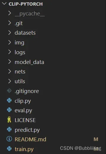
首先前往Github下载对应的仓库,下载完后利用解压软件解压,之后用编程软件打开文件夹。
注意打开的根目录必须正确,否则相对目录不正确的情况下,代码将无法运行。
一定要注意打开后的根目录是文件存放的目录。
一、数据集的准备
本文使用json格式进行训练,训练前需要自己制作好数据集,如果没有自己的数据集,可以通过Github连接下载flickr8k的数据集尝试下。
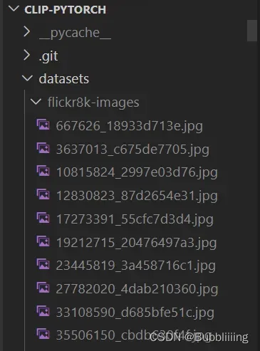
训练前将图片文件放在datasets/<数据集名称>中。
训练前将标签文件放在datasets/<标签名称>.json。
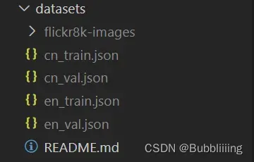
二、数据集的格式
这里我提供了两个版本的数据集,一个版本是英文的、一个版本是中文的,开头分别为en和cn。标注文件为*.json文件,*.json的格式如下,image为图片的路径,caption为对应的文本,为一个列表,内容可以多条也可以单条:
[
  {
    "image": "flickr8k-images/2513260012_03d33305cf.jpg",
    "caption": [
      "A black dog is running after a white dog in the snow .",
      "Black dog chasing brown dog through snow",
      "Two dogs chase each other across the snowy ground .",
      "Two dogs play together in the snow .",
      "Two dogs running through a low lying body of water ."
    ]
  },
  {
    "image": "flickr8k-images/2903617548_d3e38d7f88.jpg",
    "caption": [
      "A little baby plays croquet .",
      "A little girl plays croquet next to a truck .",
      "The child is playing croquette by the truck .",
      "The kid is in front of a car with a put and a ball .",
      "The little boy is playing with a croquet hammer and ball beside the car ."
    ]
  },
]
而图片文件就放在datasets/<数据集名称>中即可。
三、开始网络训练
在train.py文件里,我们有一些参数需要设置
一般而言,需要注意的参数主要为:
model_path指向需要使用到的预训练权重。
phi指向需要使用到的模型。
datasets_path为数据集存放的路径
datasets_train_json_path为训练集的标签
datasets_val_json_path为验证机的标签。
model_path和phi需要对应,本文当前支持三个模型,分别为:
"openai/VIT-B-16"
"openai/VIT-B-32"
"self-cn/VIT-B-32"
openai/VIT-B-16为openai公司开源的CLIP模型中,VIT-B-16规模的CLIP模型,英文文本与图片匹配,有公开预训练权重可用。
openai/VIT-B-32为openai公司开源的CLIP模型中,VIT-B-32规模的CLIP模型,英文文本与图片匹配,有公开预训练权重可用。
self-cn/VIT-B-32为自实现的模型,VIT-B-32规模的CLIP模型,英文文本与图片匹配,中文文本与图片匹配,无公开预训练权重可用,可以使用openai/VIT-B-32的Image Encoder初始化视觉部分,使用huggingface的bert-base-chinese初始化文本部分,进行训练时,model_path设置为model_data/ViT-B-32-OpenAI.pth即可。huggingface的bert-base-chinese会自动进行下载。
准备好数据集之后就可以开始训练了。
四、训练结果预测
训练结果预测需要用到两个文件,分别是clip.py和predict.py。
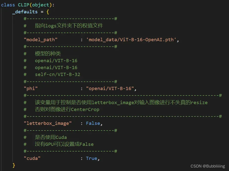
我们首先需要去clip.py里面修改model_path,在clip.py文件里面,在如下部分修改model_path使其对应训练好的文件;model_path对应logs文件夹下面的权值文件。
_defaults = {
    #-------------------------------#
    #   指向logs文件夹下的权值文件
    #-------------------------------#
    "model_path"        : 'model_data/ViT-B-16-OpenAI.pth',
    #-------------------------------#
    #   模型的种类
    #   openai/VIT-B-16
    #   openai/VIT-B-16
    #   self-cn/VIT-B-32
    #-------------------------------#
    "phi"               : "openai/VIT-B-16",
    #--------------------------------------------------------------------#
    #   该变量用于控制是否使用letterbox_image对输入图像进行不失真的resize
    #   否则对图像进行CenterCrop
    #--------------------------------------------------------------------#
    "letterbox_image"   : False,
    #-------------------------------#
    #   是否使用Cuda
    #   没有GPU可以设置成False
    #-------------------------------#
    "cuda"              : True,
}
设置好image_path和captions即可,后就可以运行predict.py进行检测了。
文章出处登录后可见!