遗传算法【Python】

遗传算法概念

基本思想：

遗传算法(GA)是一种全局寻优搜索算法，它依据的是大自然生物进化过程中“适者生存”的规律。它首先对问题的可行解进行编码，组成染色体，然后通过模拟自然界的进化过程，对初始种群中的染色体进行选择、交叉和变异，通过一代代进化来找出最优适应值的染色体来解决问题。
遗传算法是从代表问题可能潜在的解集的一个种群（population）开始的，而一个种群则由经过基因（gene）编码的一定数目的个体(individual)组成。因此，第一步需要实现从表现型到基因型的映射即编码工作。初代种群产生之后，按照适者生存和优胜劣汰的原理，逐代（generation）演化产生出越来越好的近似解，在每一代，根据问题域中个体的适应度(fitness）大小选择个体，幵借助于自然遗传学的遗传算子（genetic operators）进行组合交叉和变异，产生出代表新的解集的种群。这个过程将导致种群像自然进化一样，后生代种群比前代更加适应于环境，末代种群中的最优个体经过解码（decoding），可以作为问题近似最优解。

算子

选择算子：轮盘选择（roulette wheel selection）、排序选择（rank-based selection）、锦标赛选择（Tournament selection）；

交叉算子：单点交叉（Single-point crossover）、k点交叉（K-point crossover）、均匀交叉（Uniform crossover）等；

变异算子：位翻转突变（Flip bit mutation）、交换突变、反转突变（Swap mutation）等。

实数编码染色体的遗传算子：用于处理解空间连续问，也即个体由实数（浮点数）组成。混合交叉、模拟二进制交叉、实数突变。选择操作不受影响

快速开始

参数说明

输入：

输出：

ga.generation_best_Y 每一代的最优函数值
ga.generation_best_X 每一代的最优函数值对应的输入值
ga.all_history_FitV 每一代的每个个体的适应度
ga.all_history_Y 每一代每个个体的函数值
ga.best_y 最优函数值
ga.best_x 最优函数值对应的输入值
Y_history.index 迭代的当前次数（索引）

定义目标

import numpy as np


def schaffer(p):

    x1, x2 = p
    # x=sqe(x1)+sqr(x2)
    x = np.square(x1) + np.square(x2)
    # 0.5+((ser(sinx)-0.5) / sqr(1.0.001)*x)
    return 0.5 + (np.square(np.sin(x)) - 0.5) / np.square(1 + 0.001 * x)

运行遗传算法

from sko.GA import GA

ga = GA(func=schaffer, n_dim=2, size_pop=50, max_iter=500, prob_mut=0.001, precision=1e-7)
best_x, best_y = ga.run()
print('best_x:', best_x, '\n', 'best_y:', best_y)
# 把结果带回去测试一下

如下：

best_x: [-9.83476668e-07 -2.98023233e-08] 
 best_y: [8.8817842e-16]

注:最优解为最小值，若要求最大值，需要在前面加负号

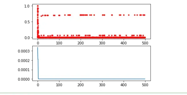
可视化

import pandas as pd
import matplotlib.pyplot as plt

Y_history = pd.DataFrame(ga.all_history_Y)
fig, ax = plt.subplots(2, 1)
ax[0].plot(Y_history.index, Y_history.values, '.', color='red')
Y_history.min(axis=1).cummin().plot(kind='line')
plt.show()

如下：

整数规划

在多维优化时，想让哪个变量限制为整数，就设定 precision 为整数即可。例如，我想让我的自定义函数 demo_func 的某些变量限制为整数+浮点数（分别是隔2个，隔1个，浮点数），那么就设定 precision=[2, 1, 1e-7]
例子如下：

from sko.GA import GA

demo_func = lambda x: (x[0] - 1) ** 2 + (x[1] - 0.05) ** 2 + x[2] ** 2
ga = GA(func=demo_func, n_dim=3, max_iter=500, lb=[-1, -1, -1], ub=[5, 1, 1], precision=[2, 1, 1e-7])
best_x, best_y = ga.run()
print('best_x:', best_x, '\n', 'best_y:', best_y)

如下：

best_x: [1.00000000e+00 0.00000000e+00 2.98023233e-08] 
best_y: [0.0025]

说明：

当 precision 为整数时，对应的自变量会启用整数规划模式。
在整数规划模式下，变量的取值可能个数最好是，这样收敛速度快，效果好。
如果 precision 不是整数（例如是0.5）,则不会进入整数规划模式，如果还想用这个模式，那么把对应自变量乘以2，这样 precision 就是整数了。

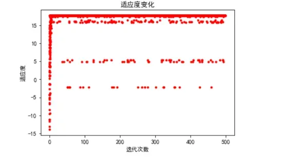
案例一：最值

题目：用标准遗传算法求函数f(x)=x+10sin(5x)+7cos(4x) 的最大值。

import numpy as np

# f(x)=x+10sin(5x)+7cos(4x) 
def schaffer(p):
     x1, x2 = p
     return x2+10*np.sin(5*x1)+7*np.cos(4*x2)



from sko.GA import GA
ga = GA(func=schaffer, n_dim=2, size_pop=50, max_iter=500, prob_mut=0.001, precision=1e-7)
best_x, best_y = ga.run()
print('x最佳值:', best_x, '\n', '最大值:', -best_y)


import pandas as pd
import matplotlib.pyplot as plt

Y_history = pd.DataFrame(ga.all_history_FitV ) #每一代的适应度
plt.rcParams['font.sans-serif']=['SimHei'] #用来正常显示中文标签
plt.rcParams['axes.unicode_minus']=False #用来正常显示负号
plt.xlabel("迭代次数")
plt.ylabel("适应度")
plt.title("适应度变化")
plt.plot(Y_history.index, Y_history.values, '.', color='red')

如下：

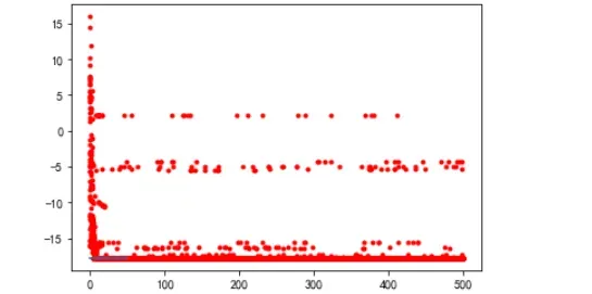
history = pd.DataFrame(ga.all_history_Y)
plt.plot(Y_history.index, history.values, '.', color='red')
history.min().cummin().plot(kind='line')
plt.show()

案例二：机器学习

以机器学习中鸢尾花的逻辑回归为例：

from sklearn.datasets import load_iris
from sklearn.linear_model import LogisticRegression
from sklearn.model_selection import train_test_split


iris = load_iris()
xtrain,xtest,ytrain,ytest = train_test_split(iris['data'],iris['target'],test_size=0.2)

def func(p):
    w1, w2 = p
    clf = LogisticRegression(max_iter=int(w1), random_state=int(w2))
    clf.fit(xtrain,ytrain)
    score = clf.score(xtest,ytest)
    return -score #由于这里的GA默认求得最小值，而我们想要score达到最大值，因此需要在score前加负号
 
ga = GA(func=func, n_dim=2, size_pop=50, max_iter=10, lb=[0, 0],ub=[3, 10],precision=1e-7)
best_x,best_y = ga.run()

print('best_x:', best_x,'\n','best_y:',best_y)

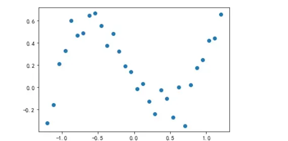
案例三：曲线拟合优化

产生x和y点：

import numpy as np
import matplotlib.pyplot as plt
from sko.GA import GA

x_true = np.linspace(-1.2, 1.2, 30)
y_true = x_true ** 3 - x_true + 0.4 * np.random.rand(30)
plt.plot(x_true, y_true, 'o')

如图：

构造参差：

def f_fun(x, a, b, c, d):
    # y=a*x^2+b*x+c*x+d
    return a * x ** 3 + b * x ** 2 + c * x + d


def obj_fun(p):
    # 四个参数,abcd
    a, b, c, d = p
    # 目标为残差
    residuals = np.square(f_fun(x_true, a, b, c, d) - y_true).sum()
    return residuals

如下：

best_x: [ 1.03756528  0.08383939 -1.02735888  0.15224675] 
best_y: [0.3521411]

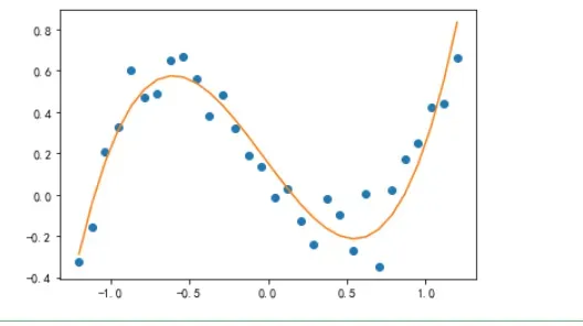
拟合：

y_predict = f_fun(x_true, *best_params)

fig, ax = plt.subplots()

ax.plot(x_true, y_true, 'o')
ax.plot(x_true, y_predict, '-')

plt.show()

如下：

参考

https://scikit-opt.github.io/scikit-opt/#/zh/curve_fitting

文章出处登录后可见！

已经登录？立即刷新