机器学习100天系列学习笔记机器学习100天(中文翻译版)机器学习100天(英文原版)
代码阅读:
第 1 步:引导包裹
#Step 1: Importing the Libraries
import numpy as np
import matplotlib.pyplot as plt
import pandas as pd
第 2 步:导入数据
#Step 2: Importing the dataset
dataset = pd.read_csv('D:/daily/机器学习100天/100-Days-Of-ML-Code-中文版本/100-Days-Of-ML-Code-master/datasets/Social_Network_Ads.csv')
X = dataset.iloc[:, [2, 3]].values
y = dataset.iloc[:, 4].values
第三步:划分训练集和测试集
#Step 3: Splitting the dataset into the Training set and Test set
from sklearn.model_selection import train_test_split
X_train, X_test, y_train, y_test = train_test_split(X, y, test_size = 0.25, random_state = 0)
第 4 步:特征缩放
#Step 4: Feature Scaling
from sklearn.preprocessing import StandardScaler
sc = StandardScaler()
X_train = sc.fit_transform(X_train)
X_test = sc.transform(X_test)
经过特征缩放后的X_train:
[[ 0.58164944 -0.88670699]
 [-0.60673761  1.46173768]
 [-0.01254409 -0.5677824 ]
 [-0.60673761  1.89663484]
 [ 1.37390747 -1.40858358]
 [ 1.47293972  0.99784738]
 [ 0.08648817 -0.79972756]
 [-0.01254409 -0.24885782]
 [-0.21060859 -0.5677824 ]...]
对于特征缩放这一步,我个人认为非常重要,它可以加快收敛速度,尤其是在深度学习的中间(梯度爆炸问题)。
第五步:Support Vector Machine
#Step 5: Fitting SVM to the Training set
from sklearn.svm import SVC
classifier = SVC(kernel = 'linear', random_state = 0)
classifier.fit(X_train, y_train)
SVC函数使用的是线性核,算法中采用的核函数类型,可选参数有:‘poly’:多项式核函数、‘rbf’:径像核函数/高斯核、‘sigmod’:sigmod核函数、‘precomputed’:核矩阵
注:precomputed表示自己提前计算好核函数矩阵,这时候算法内部就不再用核函数去计算核矩阵,而是直接用你给的核矩阵。
第 6 步:预测
#Step 6: Predicting the Test set results
y_pred = classifier.predict(X_test)
第 7 步:混淆矩阵
#Step 7: Making the Confusion Matrix
from sklearn.metrics import confusion_matrix
from sklearn.metrics import classification_report
cm = confusion_matrix(y_test, y_pred)
print(cm)  # print confusion_matrix
print(classification_report(y_test, y_pred))   # print classification report
混淆:简单理解为一个class被预测成另一个class。
给出链接混淆矩阵的参考
然后谈谈classification_report函数;科学上网,正常上网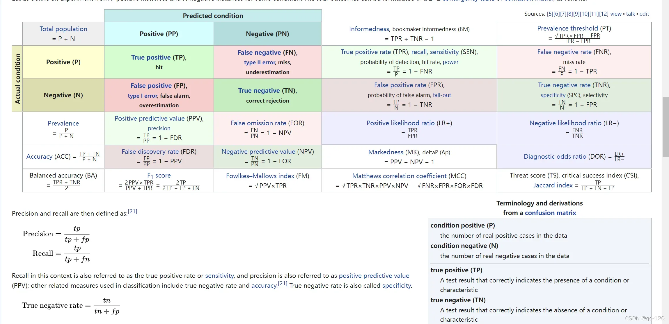
输出:
[[66  2]
 [ 8 24]]
              precision    recall  f1-score   support

           0       0.89      0.97      0.93        68
           1       0.92      0.75      0.83        32

    accuracy                           0.90       100
   macro avg       0.91      0.86      0.88       100
weighted avg       0.90      0.90      0.90       100
precision:精确度;
recall:召回率;
f1-score:precision、recall的调和函数,越接近1越好;
support:每个标签的出现次数;
avg / total行为各列的均值(support列为总和);
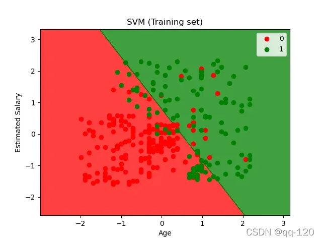
第 8 步:可视化
#Step 8: Visualization
from matplotlib.colors import ListedColormap
X_set,y_set = X_train,y_train
X1,X2 = np. meshgrid(np. arange(start=X_set[:,0].min()-1, stop=X_set[:,0].max()+1, step=0.01),
np. arange(start=X_set[:,1].min()-1, stop=X_set[:,1].max()+1, step=0.01))
plt.contourf(X1, X2, classifier.predict(np.array([X1.ravel(),X2.ravel()]).T).reshape(X1.shape),
alpha = 0.75, cmap = ListedColormap(('red', 'green')))
plt.xlim(X1.min(),X1.max())
plt.ylim(X2.min(),X2.max())
for i,j in enumerate(np.unique(y_set)):
plt.scatter(X_set[y_set==j,0],X_set[y_set==j,1],
c = ListedColormap(('red', 'green'))(i), label=j)
plt. title(' LOGISTIC(Training set)')
plt. xlabel(' Age')
plt. ylabel(' Estimated Salary')
plt. legend()
plt. show()
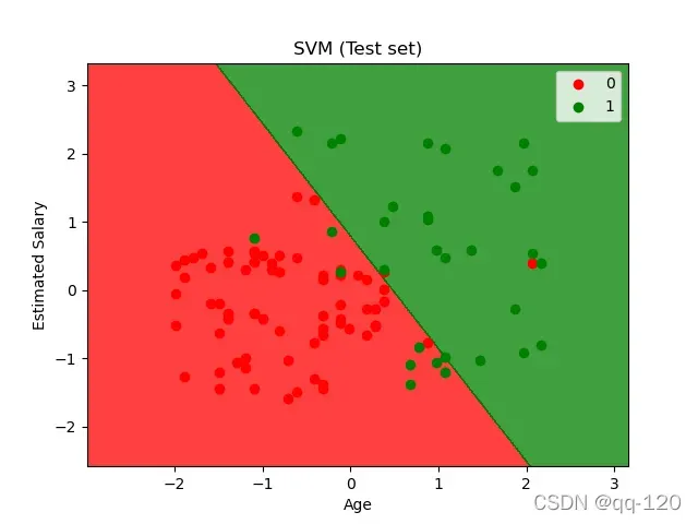
X_set,y_set=X_test,y_test
X1,X2=np. meshgrid(np. arange(start=X_set[:,0].min()-1, stop=X_set[:, 0].max()+1, step=0.01),
np. arange(start=X_set[:,1].min()-1, stop=X_set[:,1].max()+1, step=0.01))
plt.contourf(X1, X2, classifier.predict(np.array([X1.ravel(),X2.ravel()]).T).reshape(X1.shape),
alpha = 0.75, cmap = ListedColormap(('red', 'green')))
plt.xlim(X1.min(),X1.max())
plt.ylim(X2.min(),X2.max())
for i,j in enumerate(np. unique(y_set)):
plt.scatter(X_set[y_set==j,0],X_set[y_set==j,1],
c = ListedColormap(('red', 'green'))(i), label=j)
plt. title(' LOGISTIC(Test set)')
plt. xlabel(' Age')
plt. ylabel(' Estimated Salary')
plt. legend()
plt. show()
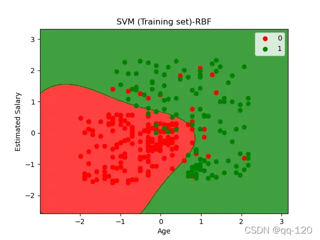
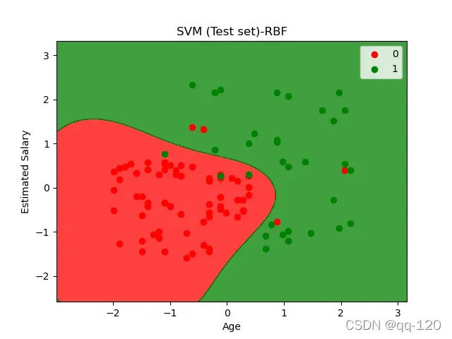
当使用RBF核时:
[[64  4]
 [ 3 29]]
              precision    recall  f1-score   support

           0       0.96      0.94      0.95        68
           1       0.88      0.91      0.89        32

    accuracy                           0.93       100
   macro avg       0.92      0.92      0.92       100
weighted avg       0.93      0.93      0.93       100
Anaconda Pytorch 实现SVM
完整代码:
#Day 5: KNN 2022/4/9
#Step 1: Importing the libraries
import numpy as np
import matplotlib.pyplot as plt
import pandas as pd

#Step 2: Importing the dataset
dataset = pd.read_csv('D:/daily/机器学习100天/100-Days-Of-ML-Code-中文版本/100-Days-Of-ML-Code-master/datasets/Social_Network_Ads.csv')
X = dataset.iloc[:, [2, 3]].values
y = dataset.iloc[:, 4].values

#Step 3: Splitting the dataset into the Training set and Test set
from sklearn.model_selection import train_test_split
X_train, X_test, y_train, y_test = train_test_split(X, y, test_size = 0.25, random_state = 0)

#Step 4: Feature Scaling
from sklearn.preprocessing import StandardScaler
sc = StandardScaler()
X_train = sc.fit_transform(X_train)
X_test = sc.transform(X_test)

#Step 5: Fitting K-NN to the Training set
from sklearn.neighbors import KNeighborsClassifier
classifier = KNeighborsClassifier(n_neighbors = 5, metric = 'minkowski', p = 2)
classifier.fit(X_train, y_train)

#Step 6: Predicting the Test set results
y_pred = classifier.predict(X_test)

#Step 7: Making the Confusion Matrix
from sklearn.metrics import confusion_matrix
from sklearn.metrics import classification_report
cm = confusion_matrix(y_test, y_pred)
print(cm)
print(classification_report(y_test, y_pred))

#Step 8: Visualization
from matplotlib.colors import ListedColormap
X_set,y_set = X_train,y_train
X1,X2 = np. meshgrid(np. arange(start = X_set[:,0].min()-1, stop = X_set[:,0].max()+1, step = 0.01),
                     np. arange(start = X_set[:,1].min()-1, stop = X_set[:,1].max()+1, step = 0.01))
plt.contourf(X1, X2, classifier.predict(np.array([X1.ravel(),X2.ravel()]).T).reshape(X1.shape),
             alpha = 0.75, cmap = ListedColormap(('red', 'green')))
plt.xlim(X1.min(),X1.max())
plt.ylim(X2.min(),X2.max())
for i,j in enumerate(np.unique(y_set)):
    plt.scatter(X_set[y_set==j,0],X_set[y_set==j,1],
                c = ListedColormap(('red', 'green'))(i), label=j)
plt. title(' LOGISTIC(Training set)')
plt. xlabel(' Age')
plt. ylabel(' Estimated Salary')
plt. legend()
plt. show()

X_set,y_set = X_test,y_test
X1,X2=np. meshgrid(np. arange(start = X_set[:,0].min()-1, stop = X_set[:,0].max()+1, step = 0.01),
                   np. arange(start = X_set[:,1].min()-1, stop = X_set[:,1].max()+1, step = 0.01))
plt.contourf(X1, X2, classifier.predict(np.array([X1.ravel(),X2.ravel()]).T).reshape(X1.shape),
             alpha = 0.75, cmap = ListedColormap(('red', 'green')))
plt.xlim(X1.min(),X1.max())
plt.ylim(X2.min(),X2.max())
for i,j in enumerate(np. unique(y_set)):
    plt.scatter(X_set[y_set==j,0],X_set[y_set==j,1],
                c = ListedColormap(('red', 'green'))(i), label=j)

plt. title(' LOGISTIC(Test set)')
plt. xlabel(' Age')
plt. ylabel(' Estimated Salary')
plt. legend()
plt. show()
文章出处登录后可见!
已经登录?立即刷新