摘要
该博客记录了一个基于numpy实现线性回归的例子。与sklearn不同,numpy实现的多为梯度下降方式优化模型性能。以下为代码部分:定义RMSE,loss,r2函数,定义回归模型,标准化,可视化等。
Import libraries
import numpy as np
import pandas as pd
import matplotlib.pyplot as plt
Define the RMSE, loss and R2 calculation functions
def rmse(y_test,pre):
    return  np.linalg.norm(y_test-pre, ord=2)/len(pre)**0.5
def R2(y_test,pre):
    return 1 - np.sum((y_test-pre)**2) / np.sum((y_test - np.mean(y_test))**2)
def Loss(y_test,pre):
    return np.sum((y_test-pre)**2)
def np_split_data(data1,n_split): # Partitioning the data set
    Y = data1.iloc[:,0]
    X = data1.iloc[:,1:]
    n = data1.shape[0]
    training_idx = list(np.random.choice(range(n),int(n*n_split),replace=False))
    # random.sample(range(1, 10), 5)
    # test_idx = numpy.random.randint(n, size=int(n*0.2))
    testing_idx = list(set(training_idx)^set(range(n)))
    # x_train,y_test = X.iloc[training_idx,:],Y.iloc[training_idx,:]
    x_train = X.iloc[training_idx,:]
    y_train  = Y.iloc[training_idx]
    x_test = X.iloc[testing_idx,:]
    y_test  = Y.iloc[testing_idx]
    x_train.index = range(x_train.shape[0])
    y_train.index = range(x_train.shape[0])
    x_test.index = range(x_test.shape[0])
    y_test.index = range(x_test.shape[0])

    return x_train,y_train,x_test,y_test
load data
path = r"/content/houseprices.csv"
data = pd.read_csv(path)
demo = data
demo
| Home | Price | SqFt | Bedrooms | Bathrooms | Offers | Brick | Neighborhood | |
|---|---|---|---|---|---|---|---|---|
| 0 | 1 | 114300 | 1790 | 2 | 2 | 2 | No | East |
| 1 | 2 | 114200 | 2030 | 4 | 2 | 3 | No | East |
| 2 | 3 | 114800 | 1740 | 3 | 2 | 1 | No | East |
| 3 | 4 | 94700 | 1980 | 3 | 2 | 3 | No | East |
| 4 | 5 | 119800 | 2130 | 3 | 3 | 3 | No | East |
| … | … | … | … | … | … | … | … | … |
| 123 | 124 | 119700 | 1900 | 3 | 3 | 3 | Yes | East |
| 124 | 125 | 147900 | 2160 | 4 | 3 | 3 | Yes | East |
| 125 | 126 | 113500 | 2070 | 2 | 2 | 2 | No | North |
| 126 | 127 | 149900 | 2020 | 3 | 3 | 1 | No | West |
| 127 | 128 | 124600 | 2250 | 3 | 3 | 4 | No | North |
128 rows × 8 columns
Different feature numerical interpolation is too large, standardized processing
from sklearn.preprocessing import StandardScaler
# Feature data encoding
size_mapping_Neighborhood = {}
for i in range(len(data["Neighborhood"].value_counts().index)):
    size_mapping_Neighborhood[data["Neighborhood"].value_counts().index[i]] = i
size_mapping_Brick = {}
for i in range(len(data["Brick"].value_counts().index)):
    size_mapping_Brick[data["Brick"].value_counts().index[i]] = i
demo["Brick"] = demo["Brick"].map(size_mapping_Brick)
demo["Neighborhood"] = demo["Neighborhood"].map(size_mapping_Neighborhood)
demo = demo.iloc[:,1:]
# Data standardization
ss = StandardScaler()
demo = ss.fit_transform(demo)
demo = pd.DataFrame(demo)
demo
| 0 | 1 | 2 | 3 | 4 | 5 | 6 | |
|---|---|---|---|---|---|---|---|
| 0 | -0.602585 | -1.000916 | -1.415327 | -0.868939 | -0.542769 | -0.698836 | -1.178538 |
| 1 | -0.606321 | 0.137904 | 1.350503 | -0.868939 | 0.396075 | -0.698836 | -1.178538 |
| 2 | -0.583903 | -1.238171 | -0.032412 | -0.868939 | -1.481614 | -0.698836 | -1.178538 |
| 3 | -1.334923 | -0.099350 | -0.032412 | -0.868939 | 0.396075 | -0.698836 | -1.178538 |
| 4 | -0.397082 | 0.612413 | -0.032412 | 1.082362 | 0.396075 | -0.698836 | -1.178538 |
| … | … | … | … | … | … | … | … |
| 123 | -0.400818 | -0.478957 | -0.032412 | 1.082362 | 0.396075 | 1.430950 | -1.178538 |
| 124 | 0.652851 | 0.754765 | 1.350503 | 1.082362 | 0.396075 | 1.430950 | -1.178538 |
| 125 | -0.632476 | 0.327707 | -1.415327 | -0.868939 | -0.542769 | -0.698836 | 0.057961 |
| 126 | 0.727580 | 0.090453 | -0.032412 | 1.082362 | -1.481614 | -0.698836 | 1.294459 |
| 127 | -0.217734 | 1.181823 | -0.032412 | 1.082362 | 1.334919 | -0.698836 | 0.057961 |
128 rows × 7 columns
x_train,y_train,x_test,y_test = np_split_data(demo,0.8)
print("x_train shape is:",x_train.shape)
print("y_train shape is:",y_train.shape)
print("x_test shape is:",x_test.shape)
print("y_test shape is:",y_test.shape)
x_train shape is: (102, 6)
y_train shape is: (102,)
x_test shape is: (26, 6)
y_test shape is: (26,)
Define the model
class LinearRegression:
def __init__(self, x_train,y_train,x_test,y_test):
# data processing
self.demo = data
self.x_train,self.y_train,self.x_test,self.y_test = x_train,y_train,x_test,y_test
self.w = np.ones(shape=(1,self.x_train.shape[1]))
# self.w[0][1:] = self.w[0][1:]*10000
self.b = np.array([[1]])
self.learningRate = 0.001
self.Loopnum = 5000
self.loss = []
def get_test_data(self):
return self.x_test,self.y_test
def predict(self,x):
predictions = np.dot(x,self.w.T)+self.b
return predictions
def train(self):
for num in range(self.Loopnum):
# print(self.w)
# B = np.array([self.b]*self.x_train.shape[0]).reshape(self.x_train.shape[0],1)
WXPlusB = np.dot(self.x_train, self.w.T) + self.b
self.y_train = np.array(self.y_train).reshape(WXPlusB.shape)
loss=np.dot((self.y_train-WXPlusB).T,self.y_train-WXPlusB)/self.y_train.shape[0]
self.loss.append(loss[0])
w_gradient = -(2/self.x_train.shape[0])*np.dot((self.y_train-WXPlusB).T,self.x_train)
# print(w_gradient)
baise_gradient = -2*np.sum(np.dot((self.x_train-WXPlusB).T,np.ones(shape=[self.x_train.shape[0],1])))/self.x_train.shape[0]
self.w=self.w-self.learningRate*w_gradient
self.b=self.b-self.learningRate*baise_gradient
def show_loss(self):
print(self.loss)
return
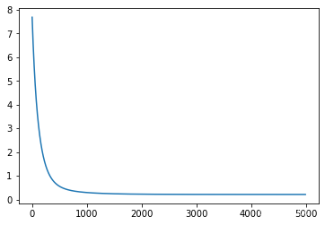
def draw(self):
plt.figure()
plt.plot(range(len(self.loss)-5),self.loss[5:])
plt.show()
return
Q1 = LinearRegression(x_train,y_train,x_test,y_test)
Q1.train()
Q1.draw()
# model.show_loss()
x_test,y_test = Q1.get_test_data() # Get the test data
from sklearn.metrics import r2_score #有自己定义的函数,效果都一样
pre = Q1.predict(x_test) # Predict prices
y_test = np.array(y_test).reshape(pre.shape)
Y_loss = np.sum((y_test-pre)**2)
# print("The single loss value is",(y_test-pre)**2)
RMSE = rmse(y_test,pre)
print("Detailed data presentation of Q1 model")
print("The test machine data house price forecast is",pre.reshape(1,len(pre)))
print("Loss value:",Y_loss)
print("RMSE:",RMSE)
print("R2 value: ", r2_score(Q1.y_train, Q1.predict(Q1.x_train)))
print("Weight vector:",Q1.w)
Detailed data presentation of Q1 model
The test machine data house price forecast is [[-9.18914099e-01 -4.36959638e-02  3.61875813e-01  6.61200258e-01
  -3.70063242e-01  9.01867176e-01  1.66935978e-04 -6.96820499e-01
  -2.24830766e-01 -6.58279255e-01 -1.23682554e-01 -6.66188042e-01
  -5.18051463e-01  3.72984245e-01 -3.21099087e-01  2.52428836e-01
   1.45079221e+00 -2.06799752e+00  1.85956363e+00  5.81677824e-01
   8.88002999e-01  7.68281468e-01 -2.28030412e-01  3.12678491e+00
  -2.14092056e-01 -4.92613761e-02]]
Loss value: 6.586735591166908
RMSE: 0.5033249291219841
R2 value:  0.7824062539612411
Weight vector: [[ 0.52005525  0.27768886  0.15460977 -0.51425199  0.26932374]]
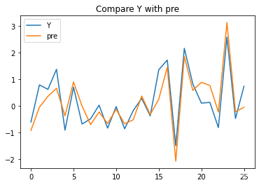
# Visualization of real and predicted data
plt.plot(range(26),y_test,label='Y')
plt.plot(range(26),pre,label='pre')
plt.title("Compare Y with pre")
plt.legend()
plt.show()
select the best model
import matplotlib.pyplot as plt
fig,ax = plt.subplots(nrows = 3,ncols = 2,figsize=(14,12))
ax[0][0].scatter(demo.iloc[:,1],demo.iloc[:,0])
ax[0][1].scatter(demo.iloc[:,2],demo.iloc[:,0])
ax[1][0].scatter(demo.iloc[:,3],demo.iloc[:,0])
ax[1][1].scatter(demo.iloc[:,4],demo.iloc[:,0])
ax[2][0].scatter(demo.iloc[:,5],demo.iloc[:,0])
ax[2][1].scatter(demo.iloc[:,6],demo.iloc[:,0])
ax[0][0].set_xlabel(data.columns[2])
ax[0][0].set_ylabel(data.columns[1])
ax[0][1].set_xlabel(data.columns[3])
ax[1][0].set_xlabel(data.columns[4])
ax[1][1].set_xlabel(data.columns[5])
ax[2][0].set_xlabel(data.columns[6])
ax[2][1].set_xlabel(data.columns[7])
plt.show()
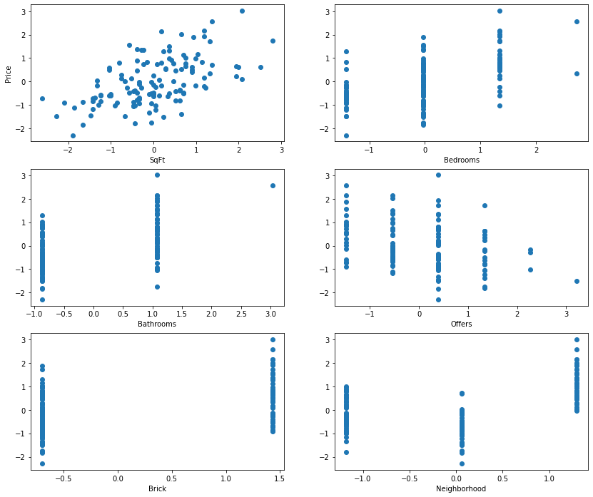
demo0 =demo.drop(demo.columns[2], axis=1)
x_train,y_train,x_test,y_test = np_split_data(demo0,0.8)
Q2 = LinearRegression(x_train,y_train,x_test,y_test)
Q2.train()
x_test,y_test = Q2.get_test_data()
pre = Q2.predict(x_test) # Predict prices
y_test = np.array(y_test).reshape(pre.shape)
Y_loss = np.sum((y_test-pre)**2)
RMSE = rmse(y_test,pre)
print("Detailed data presentation of Q2 model")
print("The test machine data house price forecast is",pre.reshape(1,len(pre)))
print("Loss value:",Y_loss)
print("RMSE:",RMSE)
print("R2 value: ", r2_score(Q2.y_train, Q2.predict(Q2.x_train)))
print("Weight vector:",Q2.w)
Detailed data presentation of Q2 model
The test machine data house price forecast is [[-0.73152743 -1.27962581  0.0920423  -0.95137815  0.55296749  0.3941641
   0.03079132 -0.83098956  0.24954459 -0.62426603 -1.43822556  0.15402153
  -1.15424147 -0.50879432  1.65785734  1.43012849 -0.25162625  0.78827719
  -0.72864504  1.20641756  0.05650989 -0.52213994 -1.15030241 -0.34219166
   1.08861407  0.07005915]]
Loss value: 4.707307862404436
RMSE: 0.4255000615748141
R2 value:  0.8447121600566533
Weight vector: [[ 0.52402705  0.20488842 -0.40842359  0.32380326  0.35594341]]
· Sorting by RMSE,Q2 subset best model < Q1 linear regression model
· Sorting by R2,Q2 subset best model>Q1 linear regression model
文章出处登录后可见!
已经登录?立即刷新