引言:
前几天被同事问到了一个问题:当batch_size=1时,Batch Normalization还有没有意义,没有说出个所以然,才意识到自己从来不好好读过BN的论文(Batch Normalization: Accelerating Deep Network Training by Reducing Internal Covariate Shift),寻思着看看可不可以从论文中得到答案,本文就是自己学习记录之用,有些狗屁不通的地方请谅解。
1. Introduce
主要分析了输入数据的分布不稳定的缺点,可以概括为两点:
原文:The change in the distributions of layers’ inputs presents a problem because the layers need to continuously adapt to the new distribution. When the input distribution to a learning system changes, it is said to experience covariate shift (Shimodaira, 2000). This is typically handled via domain adaptation (Jiang, 2008).
1. 在神经网络(Neutral network)中,对于一个神经元来说,分布不固定,会导致神经元每一次计算都要学习不同的分布,加大了训练难度,而且神经网络的级联关系,这种现象会被放大。
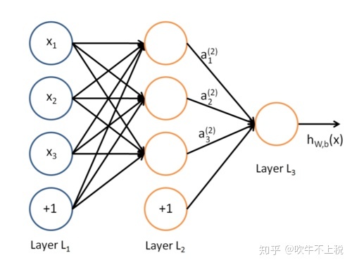
神经网络
原文:Fixed distribution of inputs to a sub-network would have positive consequences for the layers outside the subnetwork, as well. Consider a layer with a sigmoid activation function z = g(W u + b) where u is the layer input, the weight matrix W and bias vector b are the layer parameters to be learned, and g(x) = 1+exp( 1 -x). As |x| increases, g′(x) tends to zero. This means that for all dimensions of x = W u+b except those with small absolute values, the gradient flowing down to u will vanish and the model will train slowly.
2. 如果使用了sigmoid函数作为激活函数的话,因为激活函数的导数是跟x的绝对值成反比的,如果分布不固定,x的绝对值较大,那么就会梯度消失。
论文中提到的解决方法:
- 使用relu激活函数:大于零的部分是线性的,所以不会有sigmoid进入饱和区的问题
- 小心的初始化(careful initialization):如果初始化效果不好可能训练中的前几个batch就进入饱和区了
- 小的学习率:每次backpropagation时,尽可能柔和的调整参数。
2. Towards Reducing Internal Covariate Shift
本段介绍了一下什么是internal covariate shift,简单来说就是一个环节分布变化会随着网络的加深而变得越来越严重 。深度学习网络相互关联,前一层的输出就是上一层的输入,SGD的进行参数不断的更新,上一层的输出及当前层的输入的分布会不断的变化,并随着网络数据流的传播不断影响。
原文:We could consider whitening activations at every training step or at some interval, either by modifying the network directly or by changing the parameters of the optimization algorithm to depend on the network activation values (Wiesler et al., 2014; Raiko et al., 2012; Povey et al., 2014; Desjardins & Kavukcuoglu). However, if these modifications are interspersed with the optimization steps, then the gradient descent step may attempt to update the parameters in a way that requires the normalization to be updated, which reduces the effect of the gradient step. For example, consider a layer with the input u that adds the learned bias b, and normalizes the result by subtracting the mean of the activation computed over the training data: xb = x – E[x] where x = u + b, X = {x1…N } is the set of values of x over the training set, and E[x] = N1 PN i=1 xi. If a gradient descent step ignores the dependence of E[x] on b, then it will update b ← b + ∆b, where ∆b ∝ -∂ℓ/∂xb. Then u + (b + ∆b) – E[u + (b + ∆b)] = u + b – E[u + b]. Thus, the combination of the update to b and subsequent change in normalization led to no change in the output of the layer nor, consequently, the loss. As the training continues, b will grow indefinitely while the loss remains fixed. This problem can get worse if the normalization not only centers but also scales the activations. We have observed this empirically in initial experiments, where the model blows up when the normalization parameters are computed outside the gradient descent step
这一段主要说明了,如果归一化没有参与到参数优化更新过程中,会导致参数爆炸(原文中加粗部分说明超参数b的调整与x的期望无关,作者可能想表达归一化过程与参数优化过程无关吧),解决办法就是参数更新过程(偏导数计算)中要考虑到归一化(normalization)。
3. Normalization via Mini-Batch Statistics
本小节是论文中最重要的章节,主要介绍了训练/推理过程中BN的实现,推导了BN参与的反向传播的公式,BN在CNN中的应用等。
首先,LeCun et al., 1998b[1]等人提出的归一化方法如下所示:
引入超参数后的BN方法为:
自然而然的引出了下列问题:
为什么BN的最终实现中要引入超参数γ 、β?
原文:Note that simply normalizing each input of a layer may change what the layer can represent. For instance, normalizing the inputs of a sigmoid would constrain them to the linear regime of the nonlinearity. To address this, we make sure that the transformation inserted in the network can represent the identity transform(等效变换).
如果单纯的使用归一化,会影响模型的表现能力。比如说降低了模型的非线性表达能力,以sigmoid激活函数举例,BN可能将所有的输入变量限制在了sigmoid的线性区域,模型的表达能力下降。如公式(3.1)所示,加入了超参数后,我们既可以对输入尺度上变换( ),也可以对输入进行平移变换( )。而且只要我们将俩个超参数分别设定为标准差和均值,即 , 代入到公式(3.1)就可以将得到与输入一致的输出值。
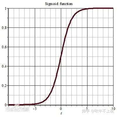
sigmoid函数
2. Batch Norm反向传播梯度计算
BN前向计算公式如下所示:
设模型损失函数为:
则BN反向传播过程,各参数的偏导数(梯度)如下:
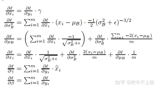
从中可以看出超参数γ和β的更新与普通参数更新是一样的,如果优化器选择梯度下降那么超参数的更新如下:
4. Training and Inference with BatchNormalized Networks
本节主要介绍了BN训练和推理(inference)过程的具体实现。
4.1 训练过程中的BN
训练过程BN计算过程如式3.3~3.7所示。代码实现[2]如下:
def batchnorm_forward(x, gamma, beta, bn_param):
  """
  Input:
  - x: (N, D)维输入数据
  - gamma: (D,)维尺度变化参数
  - beta: (D,)维尺度变化参数
  - bn_param: Dictionary with the following keys:
    - mode: 'train' 或者 'test'
    - eps: 一般取1e-8~1e-4
    - momentum: 计算均值、方差的更新参数
    - running_mean: (D,)动态变化array存储训练集的均值
    - running_var:(D,)动态变化array存储训练集的方差

  Returns a tuple of:
  - out: 输出y_i(N,D)维
  - cache: 存储反向传播所需数据
  """
  mode = bn_param['mode']
  eps = bn_param.get('eps', 1e-5)
  momentum = bn_param.get('momentum', 0.9)

  N, D = x.shape
  # 动态变量,存储训练集的均值方差
  running_mean = bn_param.get('running_mean', np.zeros(D, dtype=x.dtype))
  running_var = bn_param.get('running_var', np.zeros(D, dtype=x.dtype))

  out, cache = None, None
  # TRAIN 对每个batch操作
  if mode == 'train':
    sample_mean = np.mean(x, axis = 0)
    sample_var = np.var(x, axis = 0)
    x_hat = (x - sample_mean) / np.sqrt(sample_var + eps)
    out = gamma * x_hat + beta
    cache = (x, gamma, beta, x_hat, sample_mean, sample_var, eps)
    running_mean = momentum * running_mean + (1 - momentum) * sample_mean
    running_var = momentum * running_var + (1 - momentum) * sample_var
  # TEST:要用整个训练集的均值、方差
  elif mode == 'test':
    x_hat = (x - running_mean) / np.sqrt(running_var + eps)
    out = gamma * x_hat + beta
  else:
    raise ValueError('Invalid forward batchnorm mode "%s"' % mode)

  bn_param['running_mean'] = running_mean
  bn_param['running_var'] = running_var

  return out, cache
4.2 推理过程中的BN
推理过程中BN实现如下:
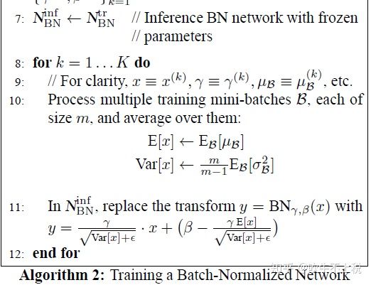
推理过程BN公式
此时自然会有一个疑问:
在推理做BN运算时,均值μ和方差σ时如何确定的?
这里原文中已经做了相应的回答,原文如下:
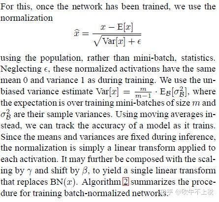
文中的大致意思是:模型训练好后,推理时Normalization使用的时总体(population)的期望和方差,而不是mini-batch的统计量。这里总体的期望和方差是使用mini-batch的无偏估计代替。总体方差的无偏估计如下所示:
这里有看不懂的同学可以参考该博文。
这里总体方差Var和期望E并不是在推理过程中确定的,而是在训练过程中确定的,训练过程中使用移动平均法更新总体方差和总体期望,训练结束后记录最终的方差和期望,在推理过程中使用该值计算BN,这样BN就是一种线性变换的方法。上述的BN实现代码中,关于Var和E(x)的更新如下所示:
 # 动态变量,存储训练集的均值方差
  running_mean = bn_param.get('running_mean', np.zeros(D, dtype=x.dtype))
  running_var = bn_param.get('running_var', np.zeros(D, dtype=x.dtype))
elif mode == 'test':
    x_hat = (x - running_mean) / np.sqrt(running_var + eps)
    out = gamma * x_hat + beta
与论文不同的是:代码实现中依旧是以式(3.6)计算的BN。
5. Batch-Normalized Convolutional Networks
故名思意BN对卷积神经网络的应用。在使用时肯定会遇到一下的一个问题:
BN是放在激活函数后还是激活函数之前?
原文:We could have also normalized the layer inputs u, but since u is likely the output of another nonlinearity, the shape of its distribution is likely to change during training, and constraining its first and second moments would not eliminate the covariate shift. In contrast, Wu+b is more likely to have a symmetric, non-sparse distribution, that is “more Gaussian” (Hyv¨arinen & Oja, 2000); normalizing it is likely to produce activations with a stable distribution。
经过非线性函数,分布有可能打乱了,经过 Wu+b可能拥有更加对称的非稀疏分布(更高斯),其经过BN可能会得到更稳定的分布。
5.1 BN在CNN中实现细节
原文:BN在CNN中的应用
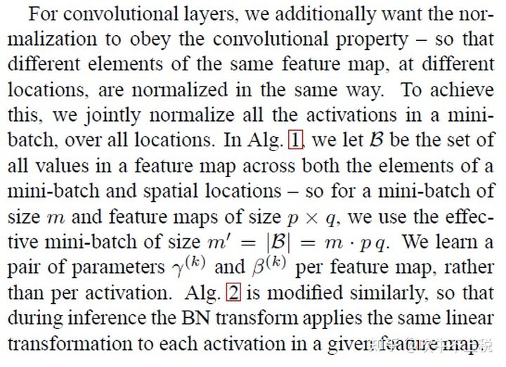
文中说了,为了使得BN能够利用CNN的特性,该特性就是参数共享(同一个特征图不同位置的不同元素公用一个参数)。因此,在CNN中同一个特征图使用统一的方法进行normalization,每个特征图学习一对儿γ,β。此时每一个特征图中BN的输入数据集合B就是特征图中的所有像素,mini-batch=m*w*h(m=batchsize,w,h为特征图的大小),样本均值μ样本方差计算公式((3.3),(3.4))中的 就是特征图中的第i个像素值(一个特征图对应一个方差和均值),normalization亦是对每一个元素进行。BN在CNN中的C++实现如下,与论文中是一致的。
void mean_cpu(float *x, int batch, int filters, int spatial, float *mean)
{
    // scale即是均值中的分母项
    float scale = 1./(batch * spatial);
    int i,j,k;
    // 外循环次数为filters,也即mean的维度,每次循环将得到一个平均值
    for(i = 0; i < filters; ++i){
        mean[i] = 0;
        // 中间循环次数为batch,也即叠加每张输入图片对应的某一通道上的输出
        for(j = 0; j < batch; ++j){
            // 内层循环即叠加一张输出特征图的所有像素值
            for(k = 0; k < spatial; ++k){
                // 计算偏移
                int index = j*filters*spatial + i*spatial + k;
                mean[i] += x[index];
            }
        }
        mean[i] *= scale;
    }
}

/*
** 计算输入x中每个元素的方差
** 本函数的主要用处应该就是batch normalization的第二步了
** x: 包含所有数据,比如l.output,其包含的元素个数为l.batch*l.outputs
** batch: 一个batch中包含的图片张数,即l.batch
** filters: 该层神经网络的滤波器个数,也即是该网络层输出图片的通道数
** spatial: 该层神经网络每张特征图的尺寸,也即等于l.out_w*l.out_h
** mean: 求得的平均值,维度为filters,也即每个滤波器对应有一个均值(每个滤波器会处理所有图片)
*/
void variance_cpu(float *x, float *mean, int batch, int filters, int spatial, float *variance)
{
    // 这里计算方差分母要减去1的原因是无偏估计,可以看:https://www.zhihu.com/question/20983193
    // 事实上,在统计学中,往往采用的方差计算公式都会让分母减1,这时因为所有数据的方差是基于均值这个固定点来计算的,
    // 对于有n个数据的样本,在均值固定的情况下,其采样自由度为n-1(只要n-1个数据固定,第n个可以由均值推出)
    float scale = 1./(batch * spatial - 1);
    int i,j,k;
    for(i = 0; i < filters; ++i){
        variance[i] = 0;
        for(j = 0; j < batch; ++j){
            for(k = 0; k < spatial; ++k){
                int index = j*filters*spatial + i*spatial + k;
                // 每个元素减去均值求平方
                variance[i] += pow((x[index] - mean[i]), 2);
            }
        }
        variance[i] *= scale;
    }
}
void normalize_cpu(float *x, float *mean, float *variance, int batch, int filters, int spatial)
{
    int b, f, i;
    for(b = 0; b < batch; ++b){
        for(f = 0; f < filters; ++f){
            for(i = 0; i < spatial; ++i){
                int index = b*filters*spatial + f*spatial + i;
                x[index] = (x[index] - mean[f])/(sqrt(variance[f]) + .000001f);
            }
        }
    }
}
/*
** axpy 是线性代数中的一种基本操作(仿射变换)完成y= alpha*x + y操作,其中x,y为矢量,alpha为实数系数,
** 请看: https://www.jianshu.com/p/e3f386771c51
** N: X中包含的有效元素个数
** ALPHA: 系数alpha
** X: 参与运算的矢量X
** INCX: 步长(倍数步长),即x中凡是INCX倍数编号的参与运算
** Y: 参与运算的矢量,也相当于是输出
*/
void axpy_cpu(int N, float ALPHA, float *X, int INCX, float *Y, int INCY)
{
    int i;
    for(i = 0; i < N; ++i) Y[i*INCY] += ALPHA*X[i*INCX];
}

void scal_cpu(int N, float ALPHA, float *X, int INCX)
{
    int i;
    for(i = 0; i < N; ++i) X[i*INCX] *= ALPHA;
}
此时的python实现应为:
mean=np.mean(x, axis=(2, 3))
var=np.var(x, axis=(2, 3))
x_hat = (x - sample_mean) / np.sqrt(sample_var + eps)
6. 引言中的疑问解答:当batch_size=1时,Batch Normalization还有没有意义,此时是不是等价于IN(instance norm)?
答:是有意义的,且与IN等价!因为在CNN中,BN的mini-batch≠batch size,而是=batchsize * w * h。假设某CNN的输入数据x的shape=[n, c, h, w],计算μ,σ时实际上的实现是:
mean=np.mean(x, axis=(2, 3))
var=np.var(x, axis=(2, 3))
该实现与IN是一致的。
Reference:
[1]. LeCun, Y., Bottou, L., Orr, G., and Muller, K. Efficient backprop. In Orr, G. and K., Muller (eds.), Neural Networks: Tricks of the trade. Springer, 1998b.
文章出处登录后可见!