序言

最近开始学习多摄融合领域了，定义是输入为多个摄像机图像，获得多个视角的相机图像特征，通过相机内外参数进行特征映射到BEV视角，得到360°的视觉感知结果，今天分享的是经典论文LSS。

论文

论文题目：《Lift, Splat, Shoot: Encoding Images from Arbitrary Camera Rigs by Implicitly Unprojecting to 3D》
lift过程：
提取图像特征，根据内外参数得到几何关系，将特征映射到BEV视角。

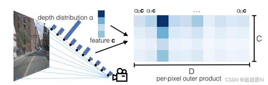
由于空间中的点有可能落到同一个像素上，造成图像深度的模糊性，因此LSS直接预测每一个采样点的深度分布，通过深度分布对相应的图像特征进行加权。每一个采样点，都有对应的加权特征，有对应的几何深度，通过内外参将其投影到BEV视角下，得到BEV空间特征。

splat过程：
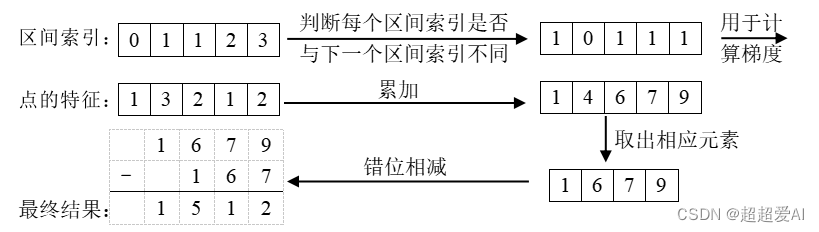
特征映射到BEV视角后，同一个BEV空间的grid存在多个采样点的图像特征，因此需要做“累加和”操作。这里采用了一个累加和小技巧，叫做“棱台池化累加和”，具体如下：

shoot过程：
对splat得到的特征进行编解码处理，实际上可以看作bev特征提取器，将编解码后的特征用于目标任务。

代码

对主要的代码进行解读：
数据读入部分：
得到多摄图像、相机内外参矩阵，以及图像增广对应的旋转和平移矩阵。

    def get_image_data(self, rec, cams):
        imgs = []
        rots = []
        trans = []
        intrins = []
        post_rots = []
        post_trans = []
        for cam in cams:
            samp = self.nusc.get('sample_data', rec['data'][cam])
            imgname = os.path.join(self.nusc.dataroot, samp['filename'])
            img = Image.open(imgname)
            post_rot = torch.eye(2)
            post_tran = torch.zeros(2)

            sens = self.nusc.get('calibrated_sensor', samp['calibrated_sensor_token'])
            intrin = torch.Tensor(sens['camera_intrinsic'])
            rot = torch.Tensor(Quaternion(sens['rotation']).rotation_matrix)
            tran = torch.Tensor(sens['translation'])

            # augmentation (resize, crop, horizontal flip, rotate)
            resize, resize_dims, crop, flip, rotate = self.sample_augmentation()
            img, post_rot2, post_tran2 = img_transform(img, post_rot, post_tran,
                                                     resize=resize,
                                                     resize_dims=resize_dims,
                                                     crop=crop,
                                                     flip=flip,
                                                     rotate=rotate,
                                                     )
            
            # for convenience, make augmentation matrices 3x3
            post_tran = torch.zeros(3)
            post_rot = torch.eye(3)
            post_tran[:2] = post_tran2
            post_rot[:2, :2] = post_rot2

            imgs.append(normalize_img(img))
            intrins.append(intrin)
            rots.append(rot)
            trans.append(tran)
            post_rots.append(post_rot)
            post_trans.append(post_tran)

        return (torch.stack(imgs), torch.stack(rots), torch.stack(trans),
                torch.stack(intrins), torch.stack(post_rots), torch.stack(post_trans))

世界坐标系下的标注信息转化到车辆坐标系下，得到对应分割的BEV视图。

    def get_binimg(self, rec):
        egopose = self.nusc.get('ego_pose',
                                self.nusc.get('sample_data', rec['data']['LIDAR_TOP'])['ego_pose_token'])
        trans = -np.array(egopose['translation'])
        rot = Quaternion(egopose['rotation']).inverse
        img = np.zeros((self.nx[0], self.nx[1]))
        for tok in rec['anns']:
            inst = self.nusc.get('sample_annotation', tok)
            # add category for lyft
            if not inst['category_name'].split('.')[0] == 'vehicle':
                continue
            box = Box(inst['translation'], inst['size'], Quaternion(inst['rotation']))
            box.translate(trans)
            box.rotate(rot)

            pts = box.bottom_corners()[:2].T
            pts = np.round(
                (pts - self.bx[:2] + self.dx[:2]/2.) / self.dx[:2]
                ).astype(np.int32)
            pts[:, [1, 0]] = pts[:, [0, 1]]
            cv2.fillPoly(img, [pts], 1.0)

        return torch.Tensor(img).unsqueeze(0)

接下来看模型代码：
看名字是建立视锥体，我觉得应该叫做create_sample_points，因为该部分代码是根据下采样倍率得到对应在输入图像上的采样点，并且在对应的采样点上补充设计的深度坐标，4到45米，41长度的深度。

    def create_frustum(self):
        # make grid in image plane
        ogfH, ogfW = self.data_aug_conf['final_dim']
        fH, fW = ogfH // self.downsample, ogfW // self.downsample
        ds = torch.arange(*self.grid_conf['dbound'], dtype=torch.float).view(-1, 1, 1).expand(-1, fH, fW)
        D, _, _ = ds.shape
        xs = torch.linspace(0, ogfW - 1, fW, dtype=torch.float).view(1, 1, fW).expand(D, fH, fW)
        ys = torch.linspace(0, ogfH - 1, fH, dtype=torch.float).view(1, fH, 1).expand(D, fH, fW)

        # D x H x W x 3
        frustum = torch.stack((xs, ys, ds), -1)
        return nn.Parameter(frustum, requires_grad=False)

这里才是真正的建立视锥体，或者也可以叫做建立视锥点云，这里其实就是位置点，和图像特征一一对应，然后对引导图像特征填入BEV空间中。

    def get_geometry(self, rots, trans, intrins, post_rots, post_trans):
        """Determine the (x,y,z) locations (in the ego frame)
        of the points in the point cloud.
        Returns B x N x D x H/downsample x W/downsample x 3
        """
        B, N, _ = trans.shape

        # undo post-transformation
        # B x N x D x H x W x 3
        points = self.frustum - post_trans.view(B, N, 1, 1, 1, 3)
        points = torch.inverse(post_rots).view(B, N, 1, 1, 1, 3, 3).matmul(points.unsqueeze(-1))

        # cam_to_ego
        points = torch.cat((points[:, :, :, :, :, :2] * points[:, :, :, :, :, 2:3],
                            points[:, :, :, :, :, 2:3]
                            ), 5)
        combine = rots.matmul(torch.inverse(intrins))
        points = combine.view(B, N, 1, 1, 1, 3, 3).matmul(points).squeeze(-1)
        points += trans.view(B, N, 1, 1, 1, 3)

        return points

因为很多位置点会落到同一个grid里面，这里会做棱台累加和的操作。最后在一个pillar求平均，这一块代码比较复杂，但做得事情很简单，

    def voxel_pooling(self, geom_feats, x):
        B, N, D, H, W, C = x.shape
        Nprime = B*N*D*H*W

        # flatten x
        x = x.reshape(Nprime, C)

        # flatten indices
        geom_feats = ((geom_feats - (self.bx - self.dx/2.)) / self.dx).long()
        geom_feats = geom_feats.view(Nprime, 3)
        batch_ix = torch.cat([torch.full([Nprime//B, 1], ix,
                             device=x.device, dtype=torch.long) for ix in range(B)])
        geom_feats = torch.cat((geom_feats, batch_ix), 1)

        # filter out points that are outside box
        kept = (geom_feats[:, 0] >= 0) & (geom_feats[:, 0] < self.nx[0])\
            & (geom_feats[:, 1] >= 0) & (geom_feats[:, 1] < self.nx[1])\
            & (geom_feats[:, 2] >= 0) & (geom_feats[:, 2] < self.nx[2])
        x = x[kept]
        geom_feats = geom_feats[kept]

        # get tensors from the same voxel next to each other
        ranks = geom_feats[:, 0] * (self.nx[1] * self.nx[2] * B)\
            + geom_feats[:, 1] * (self.nx[2] * B)\
            + geom_feats[:, 2] * B\
            + geom_feats[:, 3]
        sorts = ranks.argsort()
        x, geom_feats, ranks = x[sorts], geom_feats[sorts], ranks[sorts]

        # cumsum trick
        if not self.use_quickcumsum:
            x, geom_feats = cumsum_trick(x, geom_feats, ranks)
        else:
            x, geom_feats = QuickCumsum.apply(x, geom_feats, ranks)

        # griddify (B x C x Z x X x Y)
        final = torch.zeros((B, C, self.nx[2], self.nx[0], self.nx[1]), device=x.device)
        final[geom_feats[:, 3], :, geom_feats[:, 2], geom_feats[:, 0], geom_feats[:, 1]] = x

        # collapse Z
        final = torch.cat(final.unbind(dim=2), 1)

        return final

其他部分的代码也就比较简单了，这里不做解读了。

总结

理解代码需要储备一些坐标系转换的知识，LSS也是很经典的论文，虽然目前有各种花里胡哨的transformer论文，但自己感觉都是学术界在打榜狂欢，真正有应用价值的论文不多。但这一过程也很正常，毕竟是较新的领域，应该探索不同的途径。
LSS虽然的改进有：
1、加深度监督，比如bevdepth，目前也是sota的基本，在nuscenes检测上目前处于榜单第一。
2、还有一些特征融合的方法的改进，有人认为直接相加并不好，但这一块我没有做调研。
3、还有我自己认为的一些缺点，但目前不公开讨论，写完专利后再说。
国庆节一个人在家，宅着，学习…。唉~