目录
当你有了本领域的数据集 又有了标签 你怎么给x_train,y_train,x_test,x_test赋值呢
——自制数据集
当你数据量过少,模型见识不足,泛化力会弱
——数据增强
当每次模型训练都从0开始,很不方便
——断点续训,实时保存最优模型
神经网络训练的目的是获取各层神经网络的最优参数,只要拿到这些参数就能在其他地方快速实现神经网络的前向传播,因此需要记录这些参数
——参数提取,参数存入文本
——acc/loss可视化
——给图识物的例子
#############################################################################
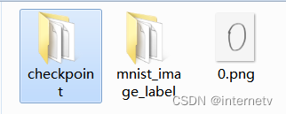
自制数据集,解决本领域应用
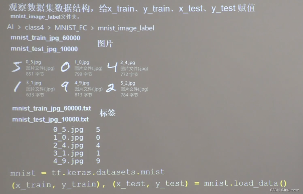
图片:黑底白字灰度图,每张图28行28列的像素点,每个像素点都是0~255之间的整数,纯黑色0,纯白色255
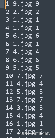
标签:txt中放的是图片名和对应的标签,中间用空格隔开
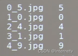
实际上txt中,
现在自写代码对x_train,y_train,x_test,x_test赋值

train_path = './mnist_image_label/mnist_train_jpg_60000/'
train_txt = './mnist_image_label/mnist_train_jpg_60000.txt'
x_train_savepath = './mnist_image_label/mnist_x_train.npy'
y_train_savepath = './mnist_image_label/mnist_y_train.npy'
test_path = './mnist_image_label/mnist_test_jpg_10000/'
test_txt = './mnist_image_label/mnist_test_jpg_10000.txt'
x_test_savepath = './mnist_image_label/mnist_x_test.npy'
y_test_savepath = './mnist_image_label/mnist_y_test.npy'
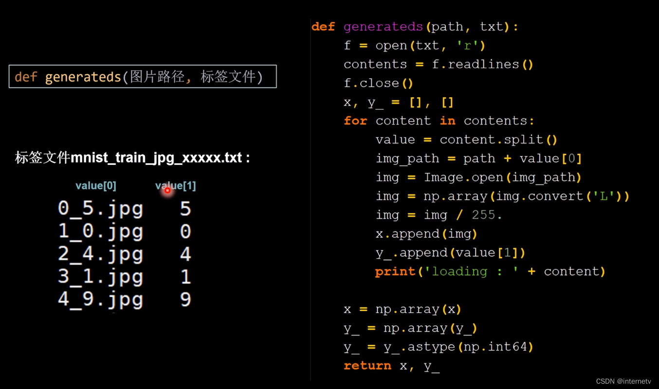
def generateds(path, txt):
f = open(txt, 'r') # 以只读形式打开txt文件
contents = f.readlines() # 读取文件中所有行
f.close() # 关闭txt文件
x, y_ = [], [] # 建立空列表
for content in contents: # 逐行取出
value = content.split() # 以空格分开,图片路径为value[0] , 标签为value[1] , 存入列表
img_path = path + value[0] # 拼出图片路径和文件名
img = Image.open(img_path) # 读入图片
img = np.array(img.convert('L')) # 图片变为8位宽灰度值的np.array格式
img = img / 255. # 数据归一化 (实现预处理)
x.append(img) # 归一化后的数据,贴到列表x
y_.append(value[1]) # 标签贴到列表y_
print('loading : ' + content) # 打印状态提示
x = np.array(x) # 变为np.array格式
y_ = np.array(y_) # 变为np.array格式
y_ = y_.astype(np.int64) # 变为64位整型
return x, y_ # 返回输入特征x,返回标签y_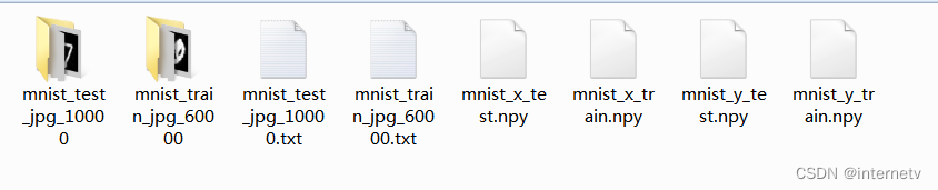
生成数据集.npy文件
总代码
import tensorflow as tf
from PIL import Image
import numpy as np
import os

train_path = './mnist_image_label/mnist_train_jpg_60000/'
train_txt = './mnist_image_label/mnist_train_jpg_60000.txt'
x_train_savepath = './mnist_image_label/mnist_x_train.npy'
y_train_savepath = './mnist_image_label/mnist_y_train.npy'

test_path = './mnist_image_label/mnist_test_jpg_10000/'
test_txt = './mnist_image_label/mnist_test_jpg_10000.txt'
x_test_savepath = './mnist_image_label/mnist_x_test.npy'
y_test_savepath = './mnist_image_label/mnist_y_test.npy'


def generateds(path, txt):
    f = open(txt, 'r')  # 以只读形式打开txt文件
    contents = f.readlines()  # 读取文件中所有行
    f.close()  # 关闭txt文件
    x, y_ = [], []  # 建立空列表
    for content in contents:  # 逐行取出
        value = content.split()  # 以空格分开,图片路径为value[0] , 标签为value[1] , 存入列表
        img_path = path + value[0]  # 拼出图片路径和文件名
        img = Image.open(img_path)  # 读入图片
        img = np.array(img.convert('L'))  # 图片变为8位宽灰度值的np.array格式
        img = img / 255.  # 数据归一化 (实现预处理)
        x.append(img)  # 归一化后的数据,贴到列表x
        y_.append(value[1])  # 标签贴到列表y_
        print('loading : ' + content)  # 打印状态提示

    x = np.array(x)  # 变为np.array格式
    y_ = np.array(y_)  # 变为np.array格式
    y_ = y_.astype(np.int64)  # 变为64位整型
    return x, y_  # 返回输入特征x,返回标签y_


if os.path.exists(x_train_savepath) and os.path.exists(y_train_savepath) and os.path.exists(
        x_test_savepath) and os.path.exists(y_test_savepath):
    print('-------------Load Datasets-----------------')
    x_train_save = np.load(x_train_savepath)
    y_train = np.load(y_train_savepath)
    x_test_save = np.load(x_test_savepath)
    y_test = np.load(y_test_savepath)
    x_train = np.reshape(x_train_save, (len(x_train_save), 28, 28))
    x_test = np.reshape(x_test_save, (len(x_test_save), 28, 28))
else:
    print('-------------Generate Datasets-----------------')
    x_train, y_train = generateds(train_path, train_txt)
    x_test, y_test = generateds(test_path, test_txt)

    print('-------------Save Datasets-----------------')
    x_train_save = np.reshape(x_train, (len(x_train), -1))
    x_test_save = np.reshape(x_test, (len(x_test), -1))
    np.save(x_train_savepath, x_train_save)
    np.save(y_train_savepath, y_train)
    np.save(x_test_savepath, x_test_save)
    np.save(y_test_savepath, y_test)

model = tf.keras.models.Sequential([
    tf.keras.layers.Flatten(),
    tf.keras.layers.Dense(128, activation='relu'),
    tf.keras.layers.Dense(10, activation='softmax')
])

model.compile(optimizer='adam',
              loss=tf.keras.losses.SparseCategoricalCrossentropy(from_logits=False),
              metrics=['sparse_categorical_accuracy'])

model.fit(x_train, y_train, batch_size=32, epochs=5, validation_data=(x_test, y_test), validation_freq=1)
model.summary()
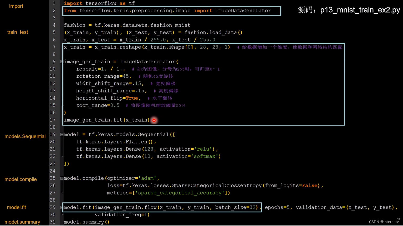
数据增强,扩充数据集

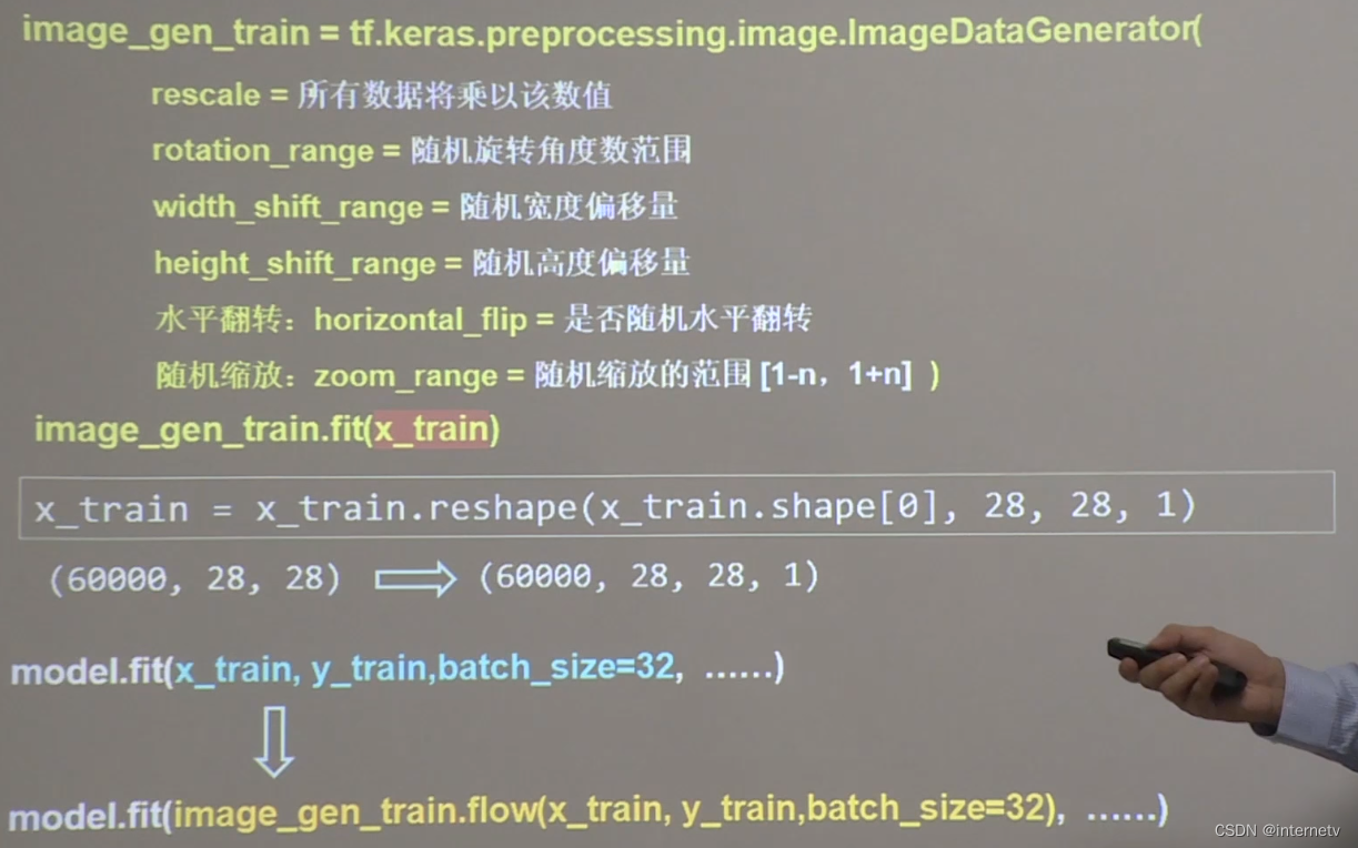
因为第4维是图片像素点颜色RGB, 有很多种表示方法,比如 rgba 四个数值表示,或者一个灰度值表示. 故统一用一个数组表示, 相比原来的数值标量, 就等于增加了一个维度 图中使用了(60000,28,28,1)即表示变成了灰度图片
1 增加维度是为了使数据和网络结构匹配,就是说 和真实的图片能一样2 增加维度的,因为可能不是灰度图片
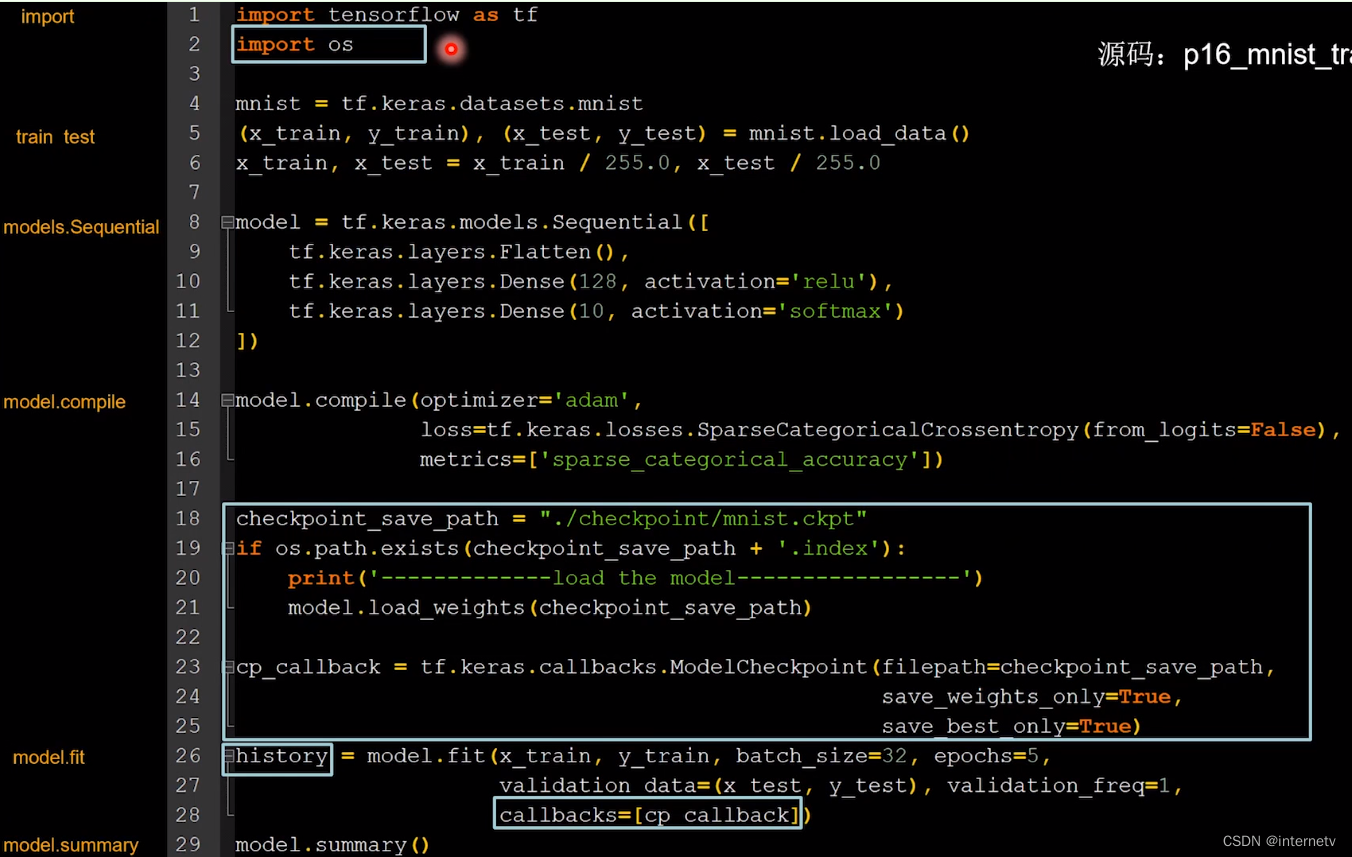
断点续训,存取模型
断点续训:在进行神经网络训练过程中由于一些因素导致训练无法进行,需要保存当前的训练结果下次接着训练

读取已有的模型
保存现有的模型
是否保留模型参数save_weights_only=True
是否保留最优模型save_best_only=True
history里储存了loss和metrics的结果,用于后面可视化
import tensorflow as tf
import os
mnist = tf.keras.datasets.mnist
(x_train, y_train), (x_test, y_test) = mnist.load_data()
x_train, x_test = x_train / 255.0, x_test / 255.0
model = tf.keras.models.Sequential([
tf.keras.layers.Flatten(),
tf.keras.layers.Dense(128, activation='relu'),
tf.keras.layers.Dense(10, activation='softmax')
])
model.compile(optimizer='adam',
loss=tf.keras.losses.SparseCategoricalCrossentropy(from_logits=False),
metrics=['sparse_categorical_accuracy'])
# 读取模型
checkpoint_save_path = "./checkpoint/mnist.ckpt"
if os.path.exists(checkpoint_save_path + '.index'):
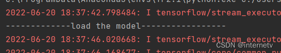
print('-------------load the model-----------------')
model.load_weights(checkpoint_save_path)
# 保存模型
cp_callback = tf.keras.callbacks.ModelCheckpoint(filepath=checkpoint_save_path,
save_weights_only=True,
save_best_only=True)
history = model.fit(x_train, y_train, batch_size=32, epochs=5, validation_data=(x_test, y_test), validation_freq=1,
callbacks=[cp_callback])
model.summary()
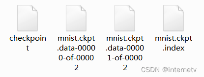
生成文件
此时再次运行程序 可以看到如图代码,说明网络是接续上一次保存的模型继续运行
参数提取,把参数存入文本
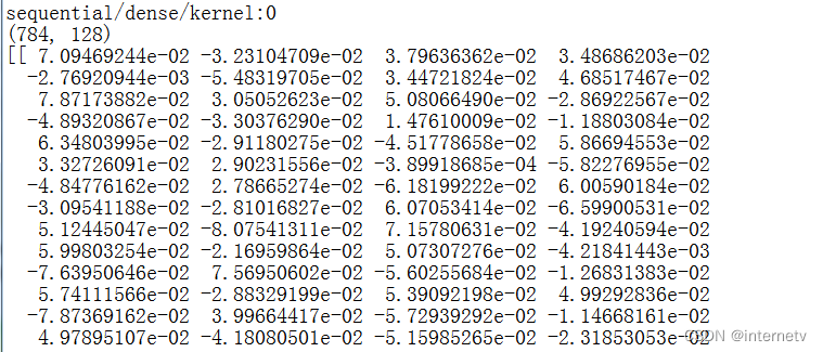
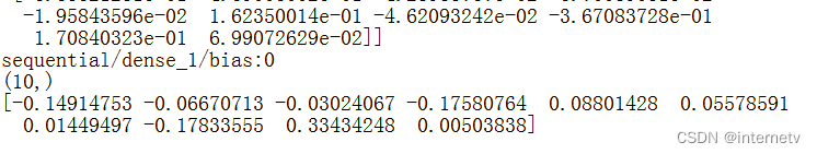
查看刚才保存的网络模型的参数
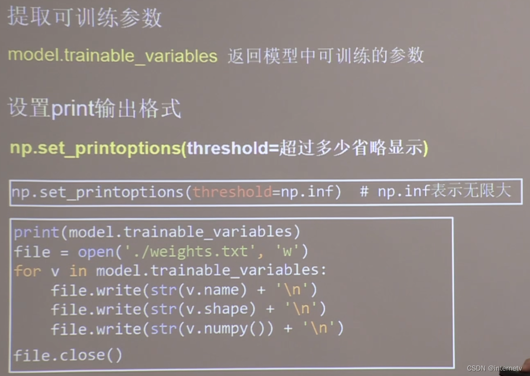
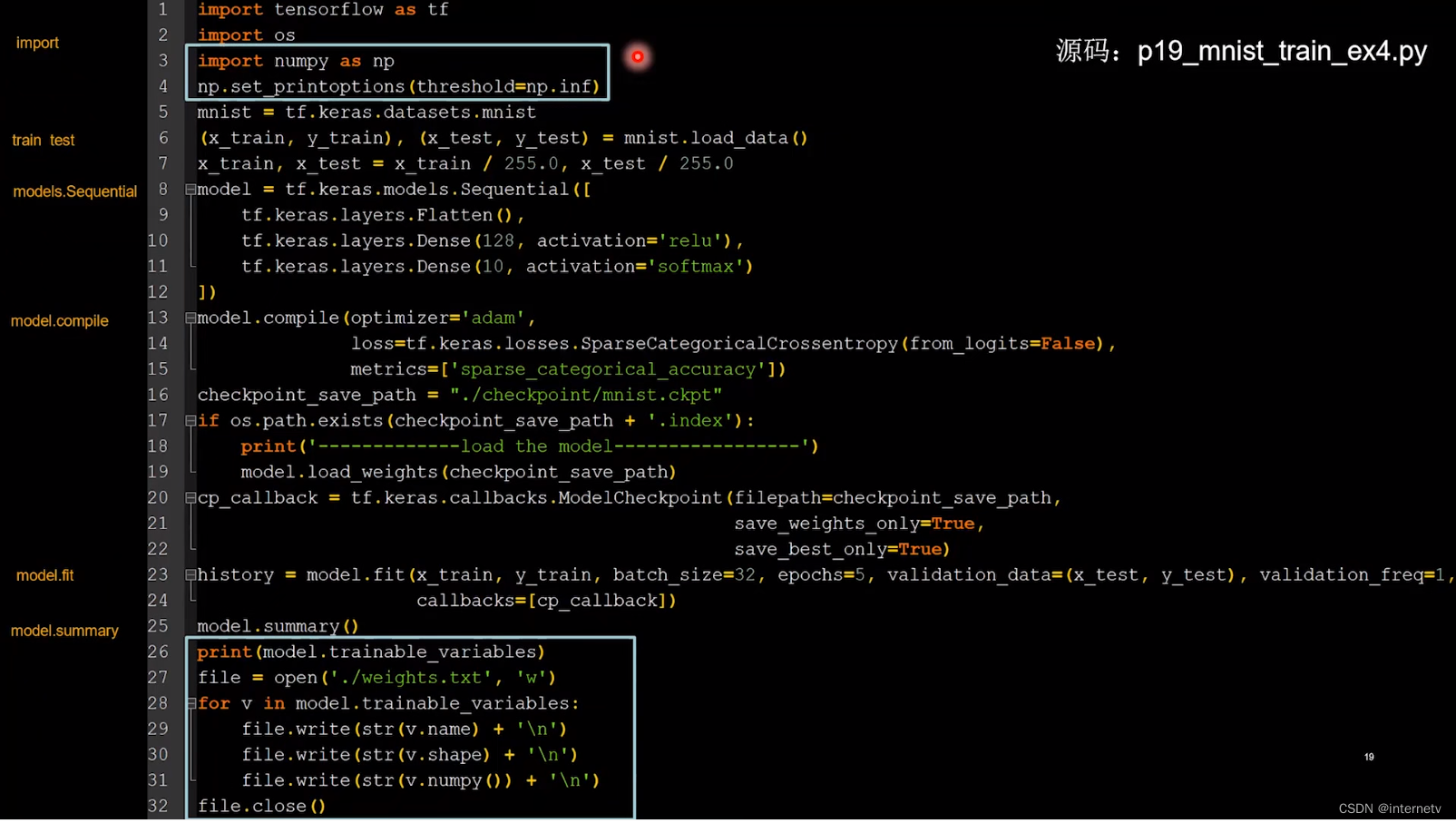
在断点续训基础上增加了参数提取 ,打印出所有参数w并存入weights.txt
import tensorflow as tf
import os
import numpy as np # 导入包
np.set_printoptions(threshold=np.inf)
mnist = tf.keras.datasets.mnist
(x_train, y_train), (x_test, y_test) = mnist.load_data()
x_train, x_test = x_train / 255.0, x_test / 255.0
model = tf.keras.models.Sequential([
    tf.keras.layers.Flatten(),
    tf.keras.layers.Dense(128, activation='relu'),
    tf.keras.layers.Dense(10, activation='softmax')
])
model.compile(optimizer='adam',
              loss=tf.keras.losses.SparseCategoricalCrossentropy(from_logits=False),
              metrics=['sparse_categorical_accuracy'])
checkpoint_save_path = "./checkpoint/mnist.ckpt"
if os.path.exists(checkpoint_save_path + '.index'):
    print('-------------load the model-----------------')
    model.load_weights(checkpoint_save_path)
cp_callback = tf.keras.callbacks.ModelCheckpoint(filepath=checkpoint_save_path,
                                                 save_weights_only=True,
                                                 save_best_only=True)
history = model.fit(x_train, y_train, batch_size=32, epochs=5, validation_data=(x_test, y_test), validation_freq=1,
                    callbacks=[cp_callback])
model.summary()
# 打印所有参数并存入weights.txt文件
print(model.trainable_variables)
file = open('./weights.txt', 'w')
for v in model.trainable_variables:
    file.write(str(v.name) + '\n')
    file.write(str(v.shape) + '\n')
    file.write(str(v.numpy()) + '\n')
file.close()
生成文件
具体内容
acc/loss可视化,查看训练效果

import tensorflow as tf
import os
import numpy as np
from matplotlib import pyplot as plt # 加入画图模块pyplot
np.set_printoptions(threshold=np.inf)
mnist = tf.keras.datasets.mnist
(x_train, y_train), (x_test, y_test) = mnist.load_data()
x_train, x_test = x_train / 255.0, x_test / 255.0
model = tf.keras.models.Sequential([
tf.keras.layers.Flatten(),
tf.keras.layers.Dense(128, activation='relu'),
tf.keras.layers.Dense(10, activation='softmax')
])
model.compile(optimizer='adam',
loss=tf.keras.losses.SparseCategoricalCrossentropy(from_logits=False),
metrics=['sparse_categorical_accuracy'])
checkpoint_save_path = "./checkpoint/mnist.ckpt"
if os.path.exists(checkpoint_save_path + '.index'):
print('-------------load the model-----------------')
model.load_weights(checkpoint_save_path)
cp_callback = tf.keras.callbacks.ModelCheckpoint(filepath=checkpoint_save_path,
save_weights_only=True,
save_best_only=True)
history = model.fit(x_train, y_train, batch_size=32, epochs=5, validation_data=(x_test, y_test), validation_freq=1,
callbacks=[cp_callback])
model.summary()
print(model.trainable_variables)
file = open('./weights.txt', 'w')
for v in model.trainable_variables:
file.write(str(v.name) + '\n')
file.write(str(v.shape) + '\n')
file.write(str(v.numpy()) + '\n')
file.close()
############################################### show ###############################################
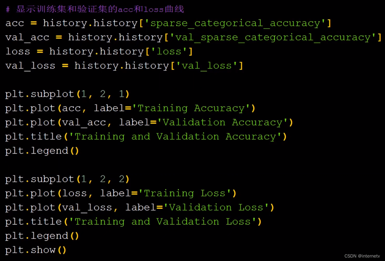
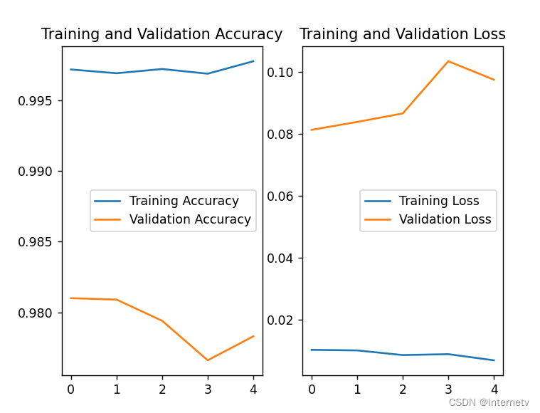
# 显示训练集和验证集的acc和loss曲线
# 提取model.fit中的训练集准确率,测试集准确率,训练集损失函数数值,测试集损失函数数值
acc = history.history['sparse_categorical_accuracy']
val_acc = history.history['val_sparse_categorical_accuracy']
loss = history.history['loss']
val_loss = history.history['val_loss']
# 划分一行两列 画出第一列
plt.subplot(1, 2, 1)
# 画出acc和val_acc数据
plt.plot(acc, label='Training Accuracy')
plt.plot(val_acc, label='Validation Accuracy')
# 设置图标题
plt.title('Training and Validation Accuracy')
# 画出图例
plt.legend()
# # 划分一行两列 画出第二列
plt.subplot(1, 2, 2)
# 画出loss和val_acc数据
plt.plot(loss, label='Training Loss')
plt.plot(val_loss, label='Validation Loss')
# 设置图标题
plt.title('Training and Validation Loss')
# 画出图例
plt.legend()
plt.show()
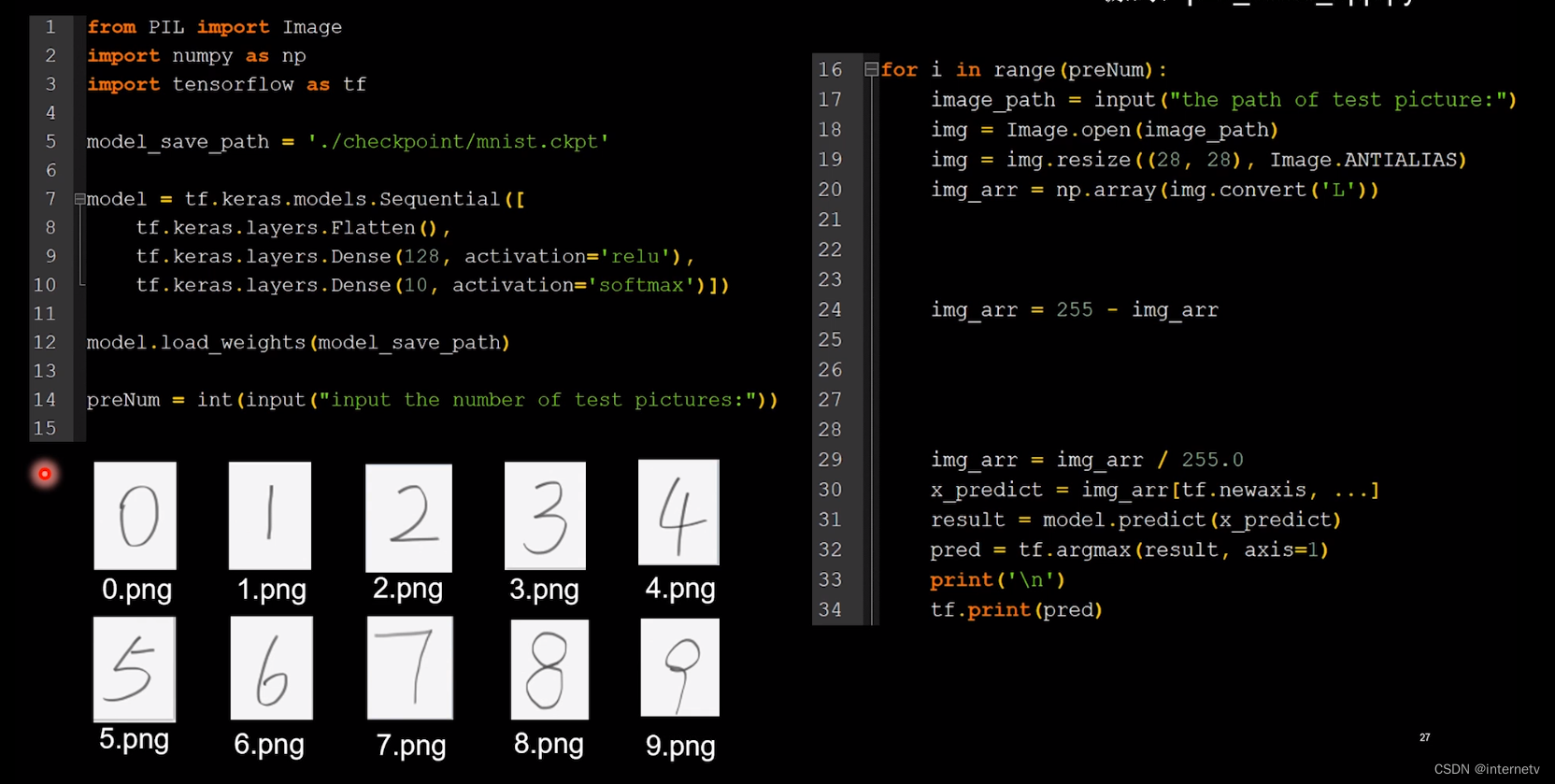
编写一个应用程序(神经网络接口),给图识物
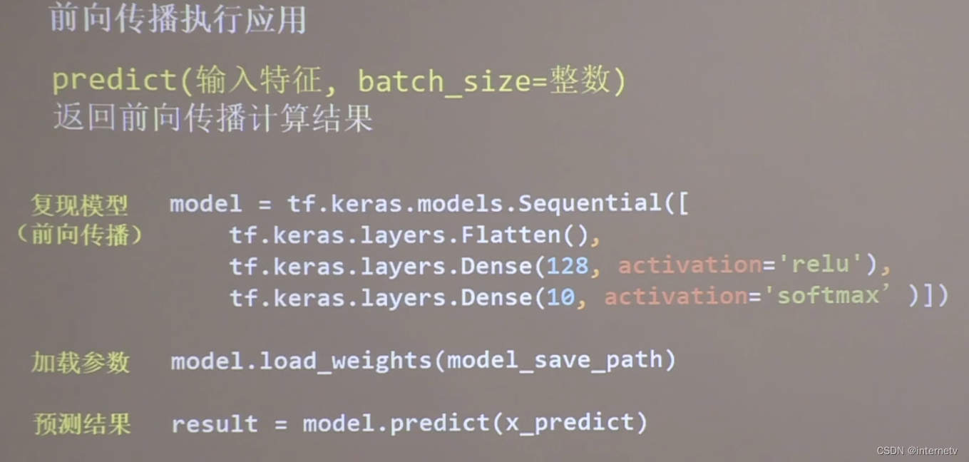
TensorFlow给了predict,他能根据输入特征,得出输出参数
预处理
灰度处理
变成只有黑色和白色的高对比度图片

把小于200的变成255,其他的变成0 —— 二值化,保留图片特征的同时,滤去了噪声,识别效果会更好
from PIL import Image
import numpy as np
import tensorflow as tf
model_save_path = './checkpoint/mnist.ckpt'
# 复现网络
model = tf.keras.models.Sequential([
tf.keras.layers.Flatten(),
tf.keras.layers.Dense(128, activation='relu'),
tf.keras.layers.Dense(10, activation='softmax')])
# 加载参数
model.load_weights(model_save_path)
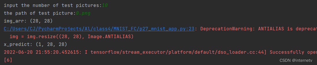
# 询问要执行多少次图像识别任务
preNum = int(input("input the number of test pictures:"))
# 读入要识别的图片
for i in range(preNum):
image_path = input("the path of test picture:")
img = Image.open(image_path)
img = img.resize((28, 28), Image.ANTIALIAS)
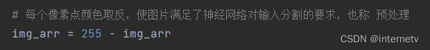
img_arr = np.array(img.convert('L'))
# 每个像素点颜色取反,使图片满足了神经网络对输入分割的要求,也称 预处理
img_arr = 255 - img_arr
# 归一化
img_arr = img_arr / 255.0
print("img_arr:",img_arr.shape)
x_predict = img_arr[tf.newaxis, ...]
print("x_predict:",x_predict.shape)
result = model.predict(x_predict)
pred = tf.argmax(result, axis=1)
print('\n')
tf.print(pred)
文章出处登录后可见!