- 原理
-
- Vanilla Transformer 与 LLaMa 的区别
- LLaMa-1/2/3 演进
- Embedding
- RMS Norm
- RoPE(Rotary Positional Encodding)
- SwiGLU Function
- KV-Cache
- Grouped Multi-Query Attention
-
-
- Multi Query Attention(MQA)
- Grouped Multi-Query Attention(GMQA)
-
- 源码
-
- RMS Norm
- RoPE (Rotary Positional Encodding)
- SwiGLU Function
- KV-Cache
- Grouped Query Attention(GQA)
- LLaMa Finetine——Alpaca、Vicuna
-
- LLaMa LoRA SFT
- Alpaca inference
原理
Vanilla Transformer 与 LLaMa 的区别
主流的大语言模型都采用了Transformer架构,它是一个基于多层Self-attention的神经网络模型。
原始的Transformer由编码器(Encoder)和解码器(Decoder)两个部分构成,同时,这两个部分也可以独立使用。
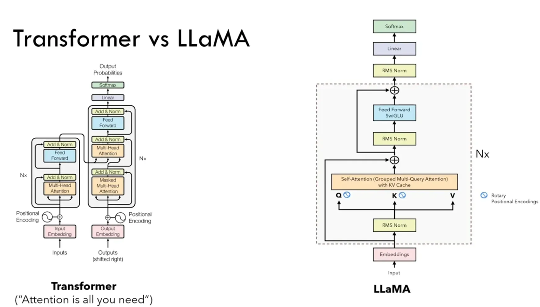
Llama模型与GPT-2类似,也是采用了基于Decoder-Only的架构。在原始Vanilla Transformer Decoder的基础上,Llama进行了如下改动:
- 为了增强训练稳定性,前置了层归一化(Pre-normalization),并使用
RMSNorm作为层归一化方法。 - 为了提高模型性能,采用
SwiGLU作为激活函数。 - 为了更好地建模长序列数据,采用
RoPE作为位置编码。 - 为了平衡效率和性能,部分模型采用了
GQA分组查询注意力机制(Grouped-Query Attention, GQA)。 - 并且将self-attention改进为使用
KV-Cache的Grouped Query。
每个版本的Llama由于其隐藏层的大小、层数的不同,均有不同的变体。接下来,我们将展开看下每个版本的不同变体。
LLaMa-1/2/3 演进
LLaMa-1系列的演进:LLaMa-1 -> Alpaca -> Vicuna 等:

-
LLaMa-1:Meta开源的Pre-trained Model,
模型参数从 7B、13B、32B、65B 不等,LLaMa-7B在大多数基准测试上超过了Text-davinci-003(即GPT3-173B),相比于ChatGPT或者GPT4来说,LLaMa可能效果上还有差距,目前hugging face已集成了LLaMa的代码实现和开源模型。学术界和工业界都可以在此基础上进行学习和研究。

-
Alpaca:斯坦福
在LLaMa-7B的基础上监督微调出来的模型,斯坦福是用OpenAI的Text-davinci-003(即GPT3-173B)的API配合self-instruct技术,使用175个提示语种子自动生成了52K条提示-回复的指示数据集,在LLaMa-7B上微调得到的模型,在8张80G的A100上训练了3小时。 -
Vicuna:
在LLaMa-13B的基础上使用监督微调得到的模型,数据集来自于ShareGPT 产生的用户对话数据,共70K条。使用Pytorch FSDP在8张A100上训练了一天。相较于Alpaca,Vicuna在训练中将序列长度由512扩展到了2048,并且通过梯度检测和flash attention来解决内存问题;调整训练损失考虑多轮对话,并仅根据模型的输出进行微调。通过GPT4来打分评测,Vicuna可以达到ChatGPT 90%的效果。
LLaMa2系列的演进:
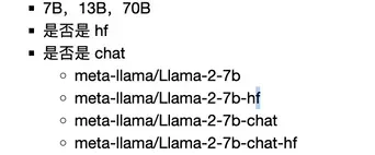
- LLaMa2:采用了Llama 1的大部分预训练设置和模型架构,有
7B、13B、34B、70B四个参数量版本。LLaMa2和LLaMa1的最大差别是:Llama-2将预训练的语料扩充到了2T token语料,同时将模型的上下文长度从2,048翻倍到了4,096,并在训练34B、70B的模型中引入了分组查询注意力机制(grouped-query attention, GQA)。

- LLaMa-2 Chat:有了更强大的基座模型Llama-2,Meta通过进一步的有监督微调(Supervised Fine-Tuning, SFT)、基于人类反馈的强化学习(Reinforcement Learning with Human Feedback, RLHF)等技术对模型进行迭代优化(
Pertrain -> SFT -> RLHF),并发布了面向对话应用的微调系列模型 Llama-2 Chat。 - Code-LLaMa:得益于Llama-2的优异性能,Meta在2023年8月发布了专注于代码生成的Code-Llama,共有7B、13B、34B和70B四个参数量版本。
LLaMa3系列的演进:
- LLaMa3:包括
8B和70B两个参数量版本。除此之外,Meta还透露,400B的Llama-3还在训练中。相比Llama-2,Llama-3支持8K长文本,并采用了一个编码效率更高的tokenizer,词表大小为128K。在预训练数据方面,Llama-3使用了超过15T token的语料,这比Llama 2的7倍还多。- 小型模型具有8B参数,其性能略优于Mistral 7B和Gemma 7B;
- 中型模型则拥有70B参数,其性能介于ChatGPT 3.5和GPT 4之间;
- 大型模型规模达到400B,目前仍在训练中,旨在成为一个多模态、多语言版本的模型,预期性能应与GPT 4或GPT 4V相当。
Embedding
Embedding的过程:word -> token_id -> embedding_vector,其中第一步转化使用tokenizer的词表进行,第二步转化使用 learnable 的 Embedding layer。

RMS Norm
对比Batch Norm 和 Layer Norm:都是减去均值Mean,除以方差Var,最终将归一化为正态分布N(0,1)。只不过两者是在不同的维度(batch还是feature)求均值和方差,(其中,减均值:re-centering 将均值mean变换为0,除方差:re-scaling将方差varance变换为1)。

RMS Norm(Root Mean Layer Norm):RMS Norm认为,Layer Norm成功的原因是re-scaling,因为方差Var计算的过程中使用了均值Mean,因此RMS Norm不再使用均值Mean,而是构造了一个特殊的统计量RMS代替方差Var。为什么使用RMS Norm?(1)RMS Norm计算量更小。(2)RMS的效果和Layer Norm一样好。
针对输入向量 a 的RMS Norm 函数计算公式如下:

此外,RMSNorm 还可以引入可学习的缩放因子gi 和偏移参数bi,从而得到
![]()
RMSNorm 在HuggingFace Transformer 库中代码实现如下所示:
class LlamaRMSNorm(nn.Module):
    def __init__(self, hidden_size, eps=1e-6):
        """
        LlamaRMSNorm is equivalent to T5LayerNorm
        """
        super().__init__()
        self.weight = nn.Parameter(torch.ones(hidden_size))
        self.variance_epsilon = eps # eps 防止取倒数之后分母为0
    def forward(self, hidden_states):
        input_dtype = hidden_states.dtype
        variance = hidden_states.to(torch.float32).pow(2).mean(-1, keepdim=True)
        hidden_states = hidden_states * torch.rsqrt(variance + self.variance_epsilon)
        # weight 是末尾乘的可训练参数, 即g_i
        return (self.weight * hidden_states).to(input_dtype)
为了使得模型训练过程更加稳定,GPT-2 相较于GPT 就提出了将Layer Norm前置,将第一个层归一化移动到多头自注意力层之前,第二个层归一化也移动到了全连接层之前,同时残差连接的位置也调整到了多头自注意力层与全连接层之后。层归一化中也采用了RMSNorm 归一化函数。
RoPE(Rotary Positional Encodding)
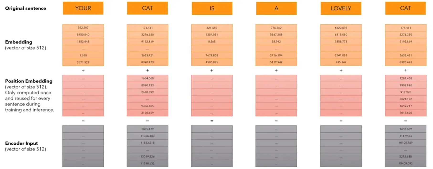
绝对Positional Encodding的使用过程:word -> token_id -> embedding_vector + position_encodding -> Encoder_Input,其中第一步转化使用tokenizer的词表进行,第二步转化使用 learnable 的 Embedding layer。将得到的embedding_vector 和 position_encodding 进行element-wise的相加,然后才做为input送入LLM的encoder。
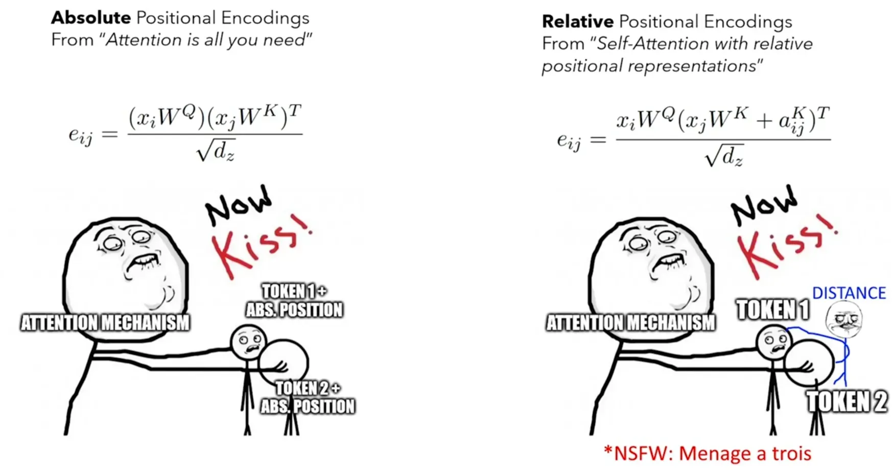
对比Absolute PE 和 Relative PE:
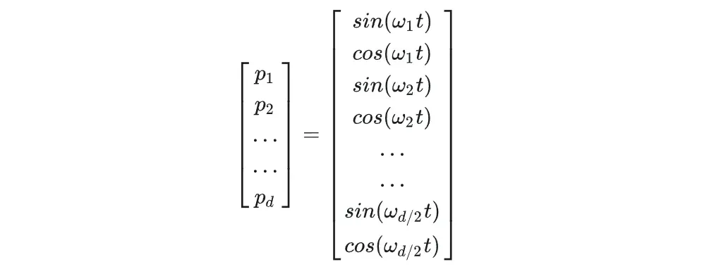
Absolute PE 绝对位置编码:每次单独1个token的PE,每个token的PE之间没有关系,是一组固定的vector,反映每个token在sequence中的绝对位置。计算 query, key 和 value 向量之前加在输入序列X上,,经典的位置编码向量 P 的计算方式是使用 Sinusoidal 函数。
Relative PE 相对位置编码:每次处理2个token的PE,只在计算attention时使用(在query@key时加在key上),反映2个token的相关度。
备注:什么是大模型外推性?(Length Extrapolation)
外推性是指大模型**在训练时和预测时的输入长度不一致,导致模型的泛化能力下降的问题。**例如,如果一个模型在训练时只使用了512个 token 的文本,那么在预测时如果输入超过512个 token,模型可能无法正确处理。这就限制了大模型在处理长文本或多轮对话等任务时的效果。
旋转位置编码(RoPE):RoPE 借助了复数的思想,出发点是通过绝对位置编码的方式,实现token间的相对位置编码。其目标是通过下述 f 运算,计算self-attention前,来给q,k 添加,其在sequence中的绝对位置信息m和n,得到qm 和kn,然后进行qm@kn:
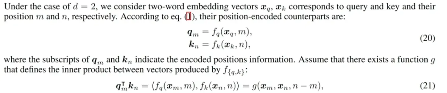
实际上,我们借助了复数的思想,寻找了一个 g 运算来合并 f 运算(分别给q和k嵌入绝对位置信息)和q@k(query和key内积)这两个操作,这样只需要给g运算输入:query,key,以及两者的在各自seqence中的绝对位置m和n,即可:

接下来的目标就是找到一个等价的位置编码方式,从而使得上述关系成立。
假定现在词嵌入向量的维度是两维 dim=2 ,这样就可以利用上2维度平面上的向量的几何性质,然后论文中提出了一个满足上述关系的 f 和 g 的形式如下(Re 表示复数的实部):
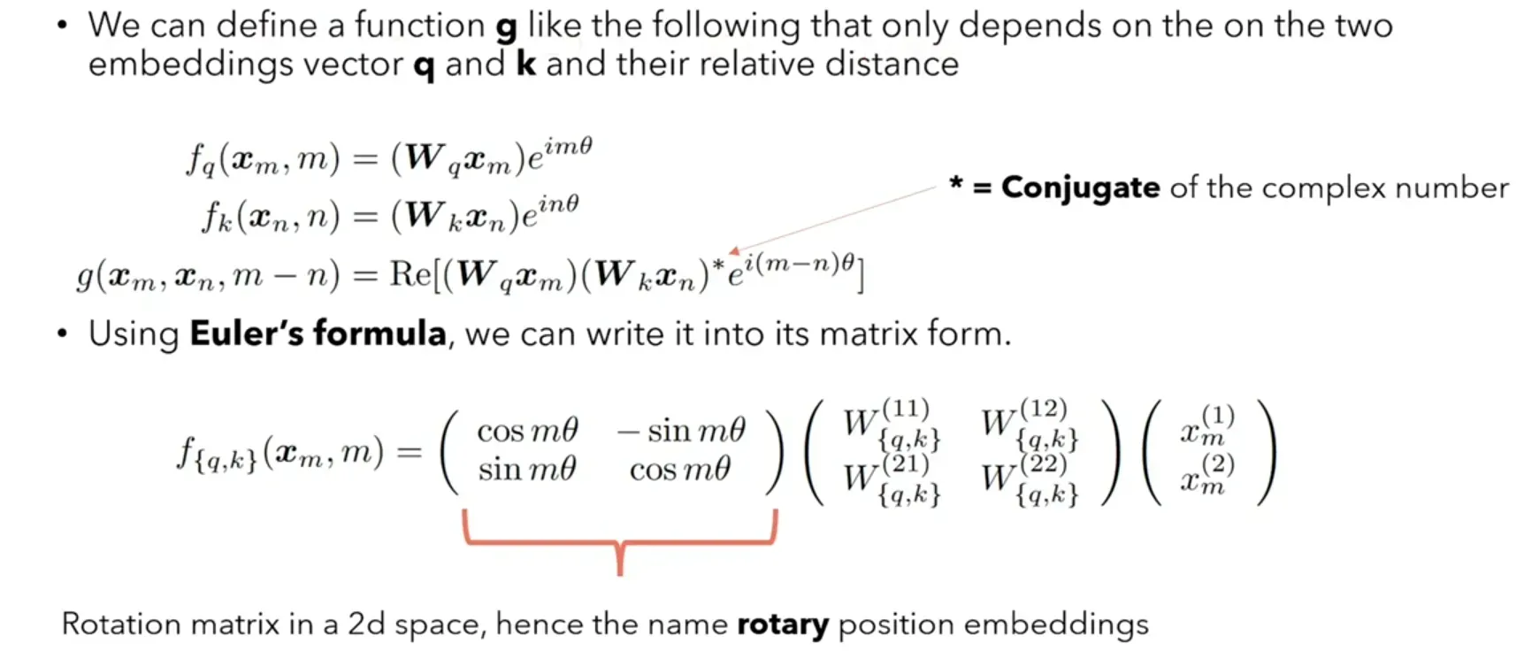
看到这里会发现,qm这不就是 q乘以了一个旋转矩阵吗?这就是为什么叫做旋转位置编码的原因。(kn也是同样)
为什么叫旋转位置编码?因为使用欧拉公式构造旋转矩阵,将分别将q和k旋转到空间中对应的位置,实现对计算结果添加位置信息,再计算qm@kn。

由于上述旋转矩阵Rn 具有稀疏性,有大量元素是0,直接用矩阵乘法来实现会很浪费算力,因此可以使用逐位相乘⊗ 操作进一步加快计算速度。从下面这个qm的实现也可以看到,RoPE 可以视为是乘性位置编码的变体。

RoPE 在HuggingFace Transformer 库中代码实现如下所示:
class LlamaRotaryEmbedding(torch.nn.Module):

    def __init__(self, dim, max_position_embeddings=2048, base=10000, device=None):
        super().__init__()
        inv_freq = 1.0 / (base ** (torch.arange(0, dim, 2).float().to(device) / dim))
        self.register_buffer("inv_freq", inv_freq)
        # Build here to make `torch.jit.trace` work.
        self.max_seq_len_cached = max_position_embeddings
        t = torch.arange(self.max_seq_len_cached, device=self.inv_freq.device,
        dtype=self.inv_freq.dtype)
        freqs = torch.einsum("i,j->ij", t, self.inv_freq)
        # Different from paper, but it uses a different permutation
        # in order to obtain the same calculation
        emb = torch.cat((freqs, freqs), dim=-1)
        dtype = torch.get_default_dtype()
        self.register_buffer("cos_cached", emb.cos()[None, None, :, :].to(dtype), persistent=False)
        self.register_buffer("sin_cached", emb.sin()[None, None, :, :].to(dtype), persistent=False)

    def forward(self, x, seq_len=None):
        # x: [bs, num_attention_heads, seq_len, head_size]
        # This `if` block is unlikely to be run after we build sin/cos in `__init__`.
        # Keep the logic here just in case.
        if seq_len > self.max_seq_len_cached:
            self.max_seq_len_cached = seq_len
            t = torch.arange(self.max_seq_len_cached, device=x.device, dtype=self.inv_freq.dtype)
            freqs = torch.einsum("i,j->ij", t, self.inv_freq)
            # Different from paper, but it uses a different permutation
            # in order to obtain the same calculation
            emb = torch.cat((freqs, freqs), dim=-1).to(x.device)
            self.register_buffer("cos_cached", emb.cos()[None, None, :, :].to(x.dtype),
            persistent=False)
            self.register_buffer("sin_cached", emb.sin()[None, None, :, :].to(x.dtype),
            persistent=False)

        return (
        self.cos_cached[:, :, :seq_len, ...].to(dtype=x.dtype),
        self.sin_cached[:, :, :seq_len, ...].to(dtype=x.dtype),
        )
    def rotate_half(x):
        """Rotates half the hidden dims of the input."""
        x1 = x[..., : x.shape[-1] // 2]
        x2 = x[..., x.shape[-1] // 2 :]
        return torch.cat((-x2, x1), dim=-1)

    def apply_rotary_pos_emb(q, k, cos, sin, position_ids):
        # The first two dimensions of cos and sin are always 1, so we can `squeeze` them.
        cos = cos.squeeze(1).squeeze(0) # [seq_len, dim]
        sin = sin.squeeze(1).squeeze(0) # [seq_len, dim]
        cos = cos[position_ids].unsqueeze(1) # [bs, 1, seq_len, dim]
        sin = sin[position_ids].unsqueeze(1) # [bs, 1, seq_len, dim]
        q_embed = (q * cos) + (rotate_half(q) * sin)
        k_embed = (k * cos) + (rotate_half(k) * sin)
        return q_embed, k_embed
SwiGLU Function
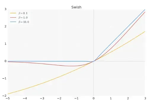
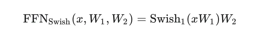
SwiGLU 激活函数是Shazeer 在文献中提出,并在PaLM等模中进行了广泛应用,并且取得了不错的效果,相较于ReLU 函数在大部分评测中都有不少提升。在LLaMA 中全连接层使用带有SwiGLU 激活函数的FFN(Position-wise Feed-Forward Network)的计算公式如下:

其中,σ(x) 是Sigmoid 函数。下图给出了Swish 激活函数在参数β 不同取值下的形状。可以看到当β 趋近于0 时,Swish 函数趋近于线性函数y = x,当β 趋近于无穷大时,Swish 函数趋近于ReLU 函数,β 取值为1 时,Swish 函数是光滑且非单调。
HuggingFace 的Transformer 库中 函数使用 SILU 函数 代替。
KV-Cache
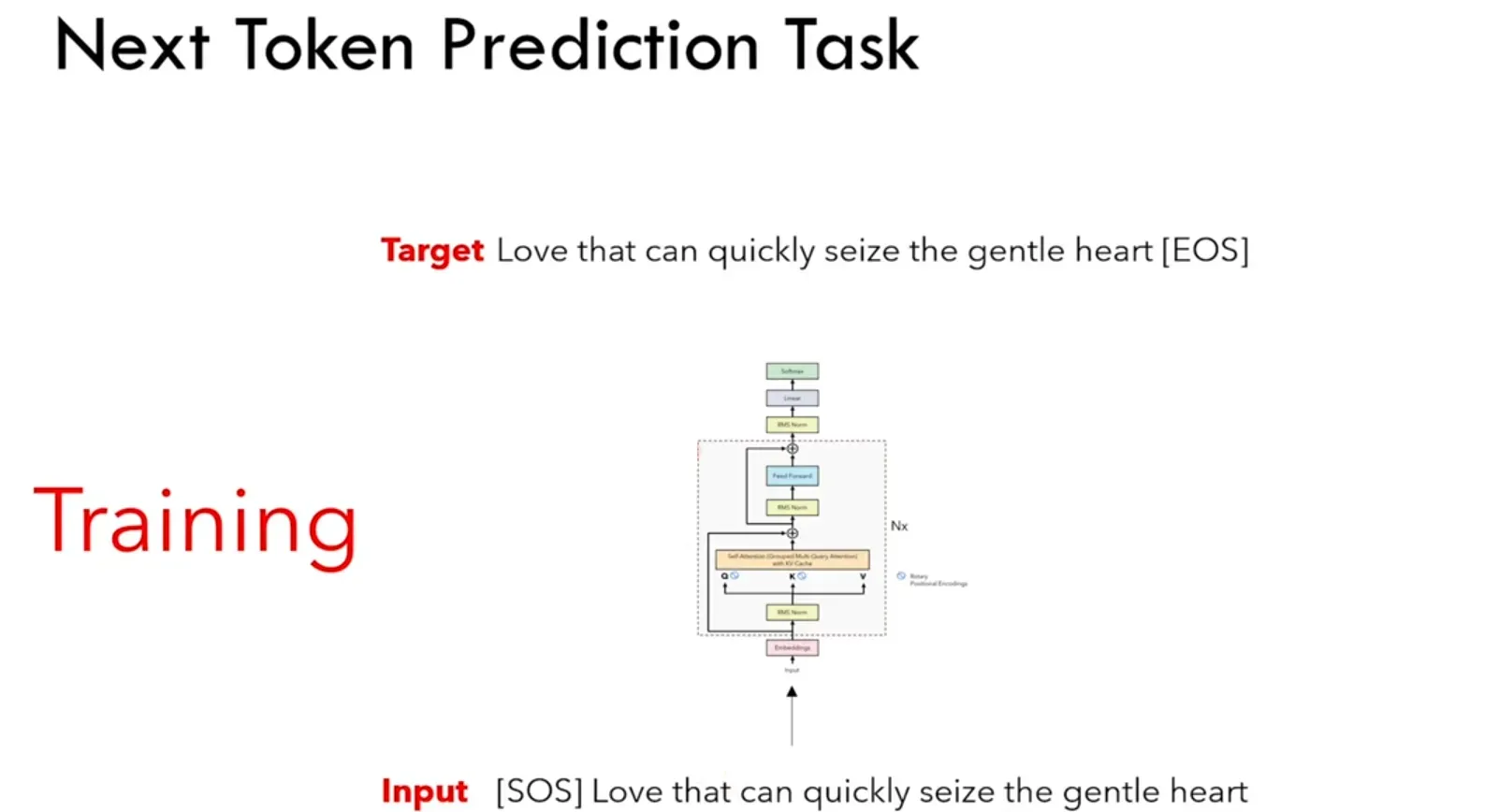
首先来了解一下LLama的训练(下词预测任务):seq2seq的生成,但迭代T次,seq_len逐渐增加。
下句预测时的Self-Attention:
- timpstep=1时
seq_len=1,给[SOS]时,预测Love;
- timpstep=2时
seq_len=2,给[SOS] 和 Love时,预测that
- timpstep=4时
seq_len=4,给[SOS] 和 Love 和 can 和 quickly时,预测seize…

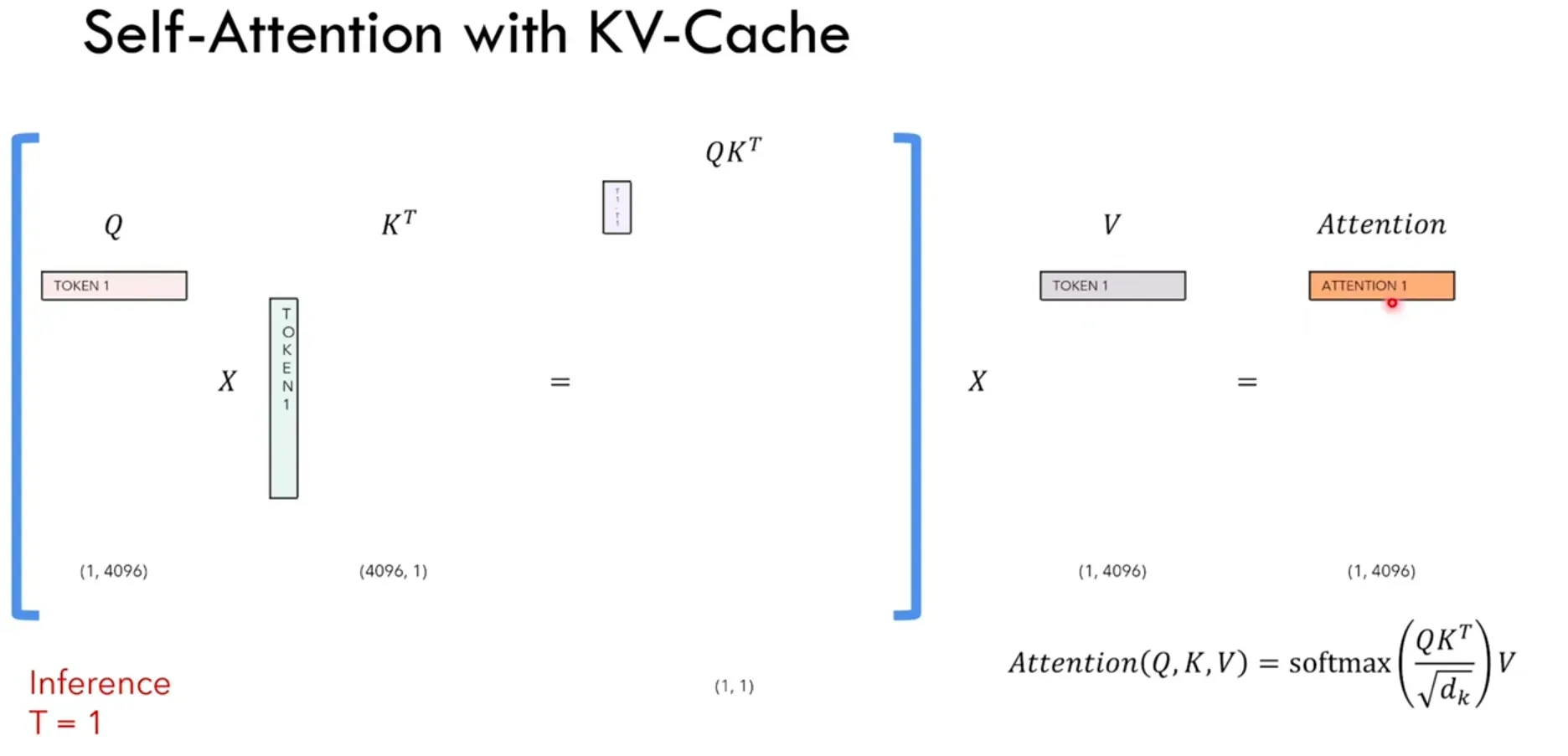
每个timestep我们只关注生成的最后一个token,但因为LLaMa是一个seq2seq的model,每次必须重新计算和生成前面的token,因此我们希望能将之前timestep计算生成过的token给缓存起来,下个timestep不用再次计算,这样的背景下,KV-Cache就产生了。
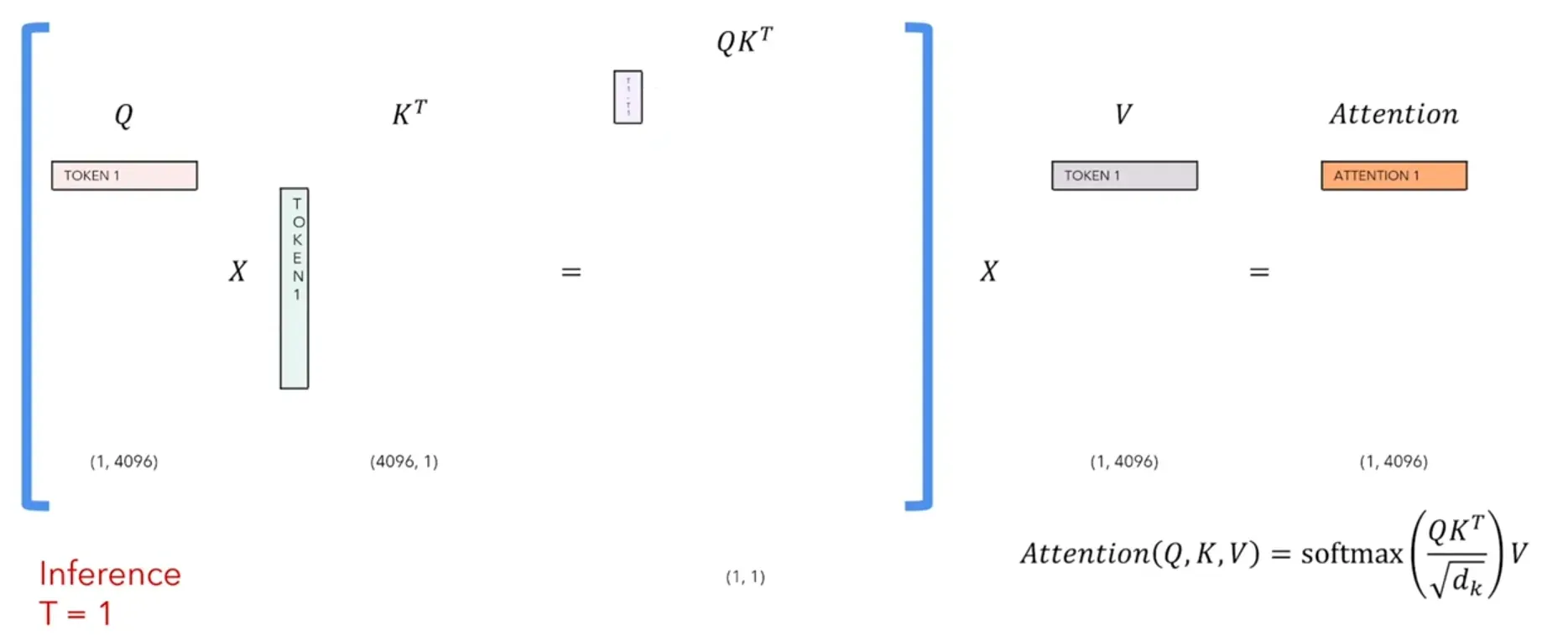
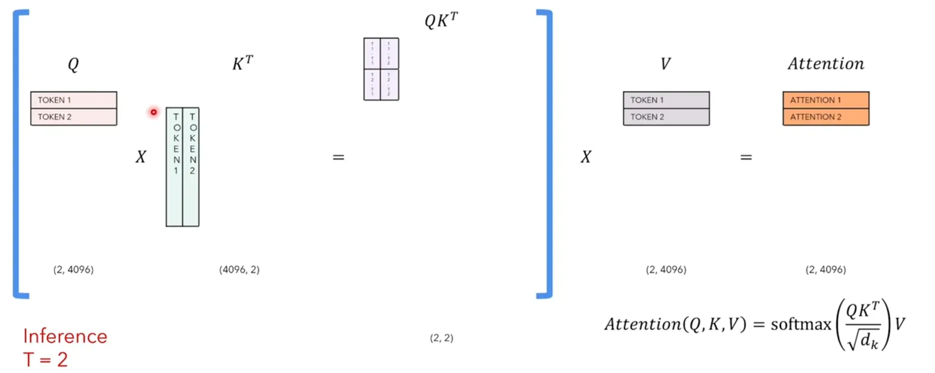
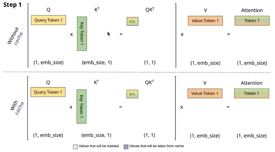
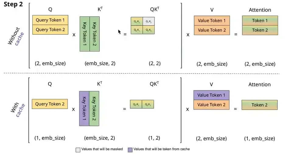
再来分析一下,每次个timestep的self-attention中我们到底需要哪些:因为我们只关注最后一个token的attention_output,如下图timestep=4,我们只需要attention_output的第4个token。
因此我们只需要Q的最后一个token和K的所有token相乘,得到最后一个token的attention_score,然后用V的所有token再与attention_score点积(相乘求和),得到最后一个token的attention_output:

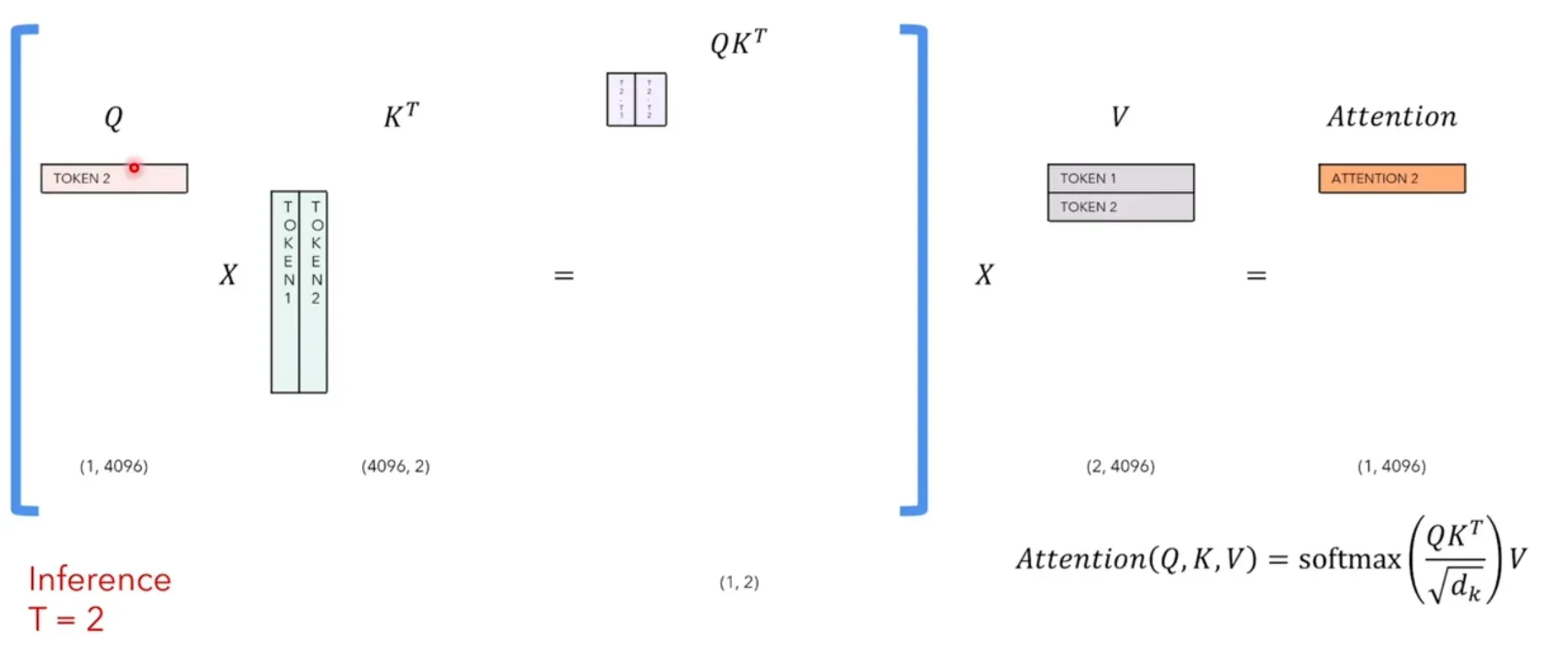
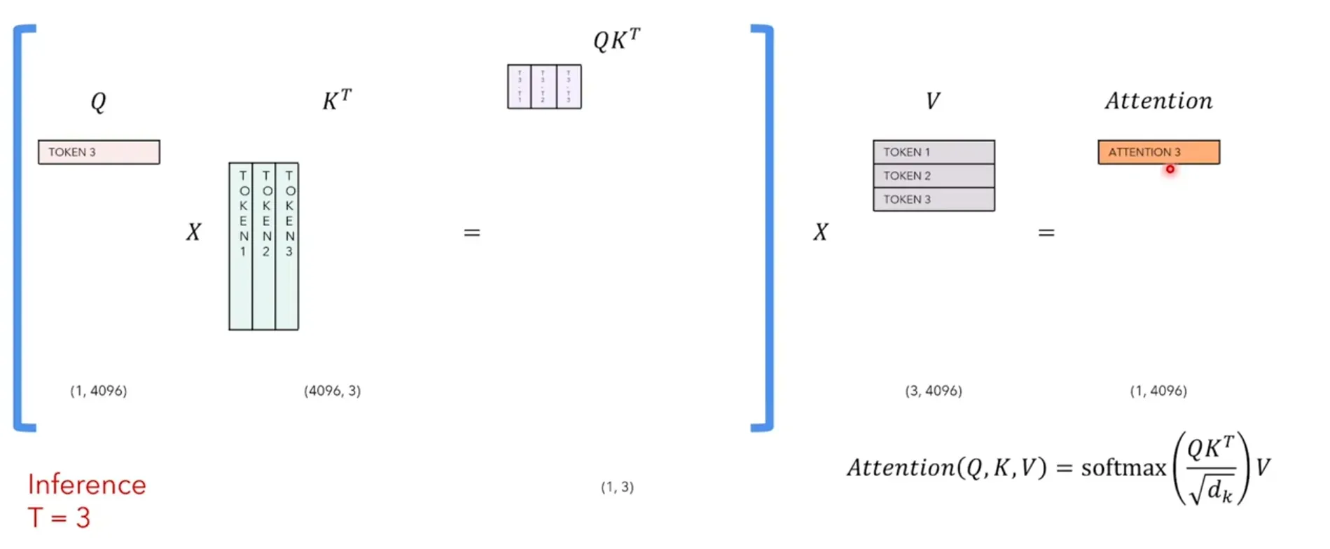
由上分析可知,每个timestep,我们的Q只需要新增的那个token即可,而K和V要缓存之前timestep的token,保证token是全的。每次计算出来的attention_output就是那个新增的token的attention。 这样就可以节省大量计算开销。
Grouped Multi-Query Attention
回顾原始的多头注意力Multi-Head Attention:时间开销的瓶颈在于矩阵的运算matrix computation。
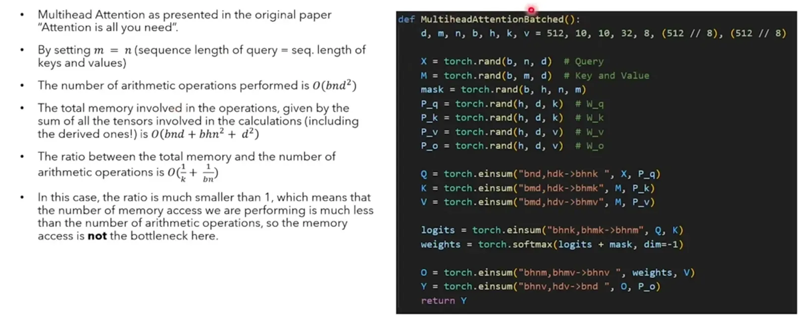
当我们使用KV-Cache后:时间开销的瓶颈在于内存的访问memory access。

Multi Query Attention(MQA)
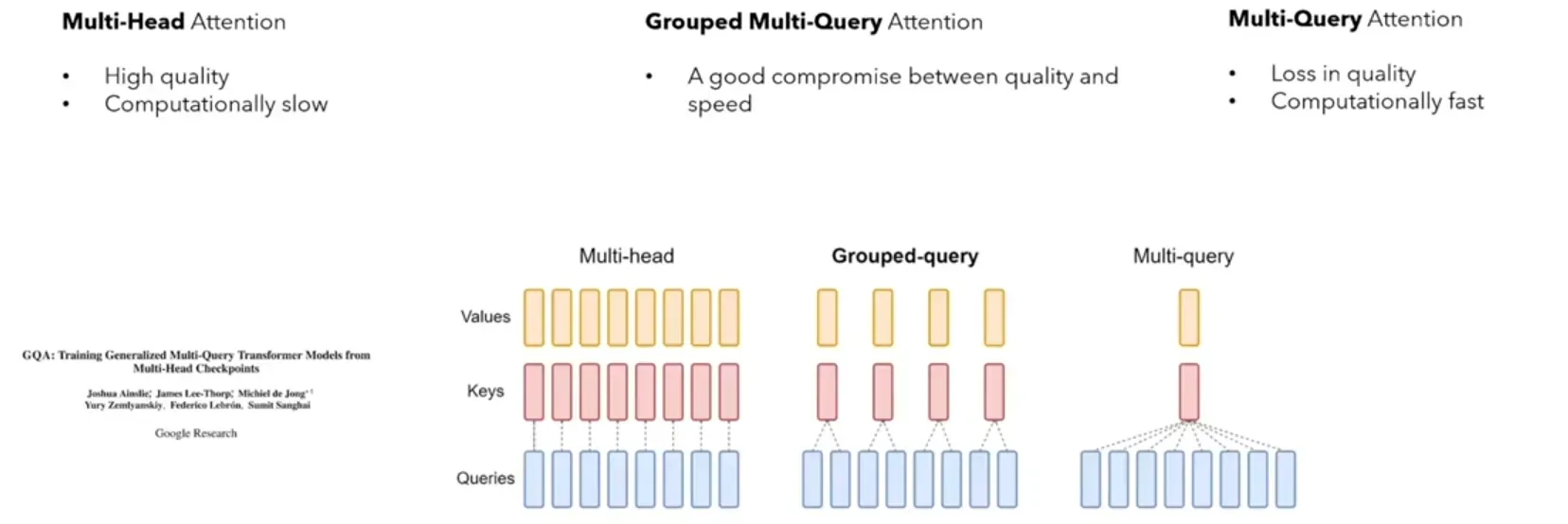
为了提升attention计算效率,多查询注意力(Multi Query Attention,MQA) 是多头注意力的一种变体。其主要区别在于,在多查询注意力中多个不同的注意力head共享一个k和v的集合,每个head只单独保留了一份q参数。 具体操作上,去除 K和V 的head维度,只为Q保留head维度。因此这就是被叫做Multi Query Attention的原因。

因此K和V的矩阵的数量仅为1个(不分head),大幅度减少了显存占用,使其更高效。由于多查询注意力改变了注意力机制的结构,因此模型通常需要从训练开始就支持多查询注意力。
研究结果表明,可以通过对已经训练好的模型进行微调来添加多查询注意力支持,仅需要约 5% 的原始训练数据量就可以达到不错的效果。包括Falcon、SantaCoder、StarCoder等在内很多模型都采用了多查询注意力机制。
Grouped Multi-Query Attention(GMQA)
就是在 Multi-Query Attention的基础上,对input进行分组,如下图2个head分为1组,每组都有自己的K,V,每个组包含2个Q。 (与MQA的区别在于:MQA的KV只有1份;GQA的KV有group份(LLama-70B中是kv_heads=8,即每个kv对应8个q))

import torch
import torch.nn as nn
from torch.nn import functional as F
from typing import Optional

x = torch.rand(1, 512, 768)
batch, seq_len, d_model = x.shape
xq, xk, xv = self.wq(x), self.wk(x), self.wv(x)
query = xq.view(batch, seq_len, self.n_heads, self.head_dim).transpose(1, 2)
key = xk.view(batch, seq_len, self.n_kv_heads, self.head_dim).transpose(1, 2)
value = xv.view(batch, seq_len, self.n_kv_heads, self.head_dim).transpose(1, 2)

# repeat kv heads if n_kv_heads < n_heads
key = key.reshape(1, 1, self.n_heads//self.n_kv_heads, 1)
value = value.reshape(1, 1, self.n_heads//self.n_kv_heads, 1)

# excute scaled dot product attention
attn_score = torch.matmul(query, key.transpose(-2, -1))
attn_score = attn_score / self.scale
attn_score = torch.softmax(attn_score, dim=-1)
attn_score = self.dropout(attn_score)
attn_output = torch.matmul(attn_score, value)
attn_output = attn_output.transpose(1, 2).reshape(batch, seq_len, self.head_dim)
源码
[LLMs 实践] 01 llama、alpaca、vicuna 整体介绍及 llama 推理过程
RMS Norm
import numpy as np
import torch
from torch import nn

bs, seq_len, emb_dim = 20, 5, 10  # 20个样本, 每个样本5个token(word/patch),每个token(word/patch)是长度为10的embedding
x = torch.randn(bs, seq_len, emb_dim)
- LN (Layer Norm) 先
re-centering(减均值),再re-scaling(除方差):。LN 作用在
emb_dim维度上,使得每个embedding的均值=0,标准差=1。
ln = nn.LayerNorm(emb_dim)  # LN 作用在emb_dim维度
x_ln = ln(x)
print(x_ln[1, 4, :].mean())
print(x_ln[1, 4, :].std())
# tensor(-1.6391e-08, grad_fn=<MeanBackward0>)
# tensor(1.0541, grad_fn=<StdBackward0>)
- RMS Norm (省略了LN的
re-centering)只进行re-scaling:对于向量x,,where
。RMS Norm 也作用在
emb_dim维度上,使得每个embeddin的标准差=1。
import torch
import torch.nn as nn
class RMSNorm(torch.nn.Module):
    def __init__(self, dim, eps=1e-8):
        super().__init__()
        self.eps = eps
        self.weight = nn.Parameter(torch.ones(dim))  # 缩放因子g

    def _norm(self, x):
        return x * torch.rsqrt(x.pow(2).mean(-1, keepdim=True) + self.eps)

    def forward(self, x):
        output = self._norm(x.float().type_as(x))
        return output * self.weight

rms_norm = RMSNorm(emb_dim)
x_rms = rms_norm(x)
print(x_rms[1, 4, :].mean())
print(x_rms[1, 4, :].std())
# tensor(-0.0725, grad_fn=<MeanBackward0>)
# tensor(1.0513, grad_fn=<StdBackward0>)
torch.rsqrt(x)就是
RoPE (Rotary Positional Encodding)
Huggingface和meta实现了两版不同的RoPE,就是把复数位置信息快速融入query和key中,破坏Transformer结构中sequence的完全对称性,使得对token位置敏感。
Sinusoidal绝对位置编码(正余弦):分别计算奇数和偶数的位置编码,然后拼接在一起。
import torch.nn as nn
import math
class SinusoidalPositionEncoding(nn.Module):
    def __init__(self, dim, seq_len=5000):
        super(SinusoidalPositionEncoding, self).__init__()
        pe = torch.zeros(seq_len, dim)  # [seq_len, dim]
        position = torch.arange(0, seq_len, dtype=torch.float).unsqueeze(1)  # [seq_len, 1]
        # div_term 先算偶数,再用偶数反推奇数
        div_term = torch.exp(torch.arange(0, dim, 2).float() * (-math.log(10000.0) / dim)) # [dim/2]
        pe[:, 0::2] = torch.sin(position * div_term)  # even_pe: [seq_len, dim/2]
        pe[:, 1::2] = torch.cos(position * div_term)  # odd_pe: [seq_len, dim/2]
        # torch.Size([seq_len, dim])
        pe = pe.unsqueeze(0).transpose(0, 1)
        # torch.Size([seq_len, 1, dim])
        self.register_buffer('pe', pe)

    def forward(self, x):
        return x + self.pe[:x.size(0), :]

sinusoidal_pe = SinusoidalPositionEncoding(6, 10)
print(sinusoidal_pe.pe.shape) # torch.Size([10, 1, 6])

RoPE旋转位置编码(改进版):
- 预计算旋转矩阵
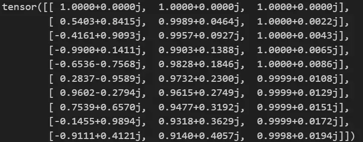
precompute_freqs_cis:计算出了i=[1,2,...,seqlen]位置的正余弦,并以复数形式表示,
实部代表偶数,虚部代表奇数。 其中cis(x)=cos(x)+i·sin(x)
import torch
import torch.nn as nn
def precompute_freqs_cis(dim: int, end: int, theta: float = 10000.0):
    """
    Args:
        dim (int): token的维度
        end (int): 通常是seqlen
        theta (float, optional): 根据公式,默认为10000

    Returns:
        torch.Tensor: 预先计算好的复数张量
    """
	# 计算词向量元素两两分组之后,每组元素对应的旋转角度\theta_i
    freqs = 1.0 / (theta ** (torch.arange(0, dim, 2)[: (dim // 2)].float() / dim))  # freqs.shape = [seq_len, dim // 2]
    # # 生成 token 序列索引 t = [0, 1,..., seq_len-1]
    t = torch.arange(end, device=freqs.device)  # t.shape = [end]
    # 这里.outer()是外积,freqs是类似正弦编码的形式,它只有dim/2维,t是包括了最大position,也就是end变量,例如在BERT中一般是512
    # 因此两个向量进行外积得到一个矩阵,维度为[end, dim/2],对应论文中的mθ,其中m代表绝对位置
    freqs = torch.outer(t, freqs).float()  # 计算 m * \theta
    # 转为复数向量,polar()函数用的很少,这一步之后实际上就算出了每一个位置m处的cosθ和sinθ的值,方便后续用于快速计算,这里具体形式可以参考上面发的文章
    # 简单来说就是每一行对应一个位置m,总共有dim/2列,每一列是该位置处的cosθi + isinθi,是一个复数向量
    freqs_cis = torch.polar(torch.ones_like(freqs), freqs) # # torch.Size([10, 3])
    return freqs_cis

precompute_freqs_cis(dim=6, end=10)
# # torch.Size([10, 3])
可以看出旋转位置编码使用复数表示,对比前面的SinCos位置编码,实部代表偶数,虚部代表奇数。 cos和sin都在一个数中,因此旋转位置编码比绝对的SinCos位置编码要少一半。
- 施加RoPE信息
apply_rotary_emb:计算query_rope时直接使用xq_ * freqs_cis,也就是按位相乘(RoPE是乘性位置编码x*p,不同于Sinusoidal那种加性位置编码x+p)。apply_rotary_emb得到含有位置信息的sequencexq和xk。
from typing import Tuple

def apply_rotary_emb(
    xq: torch.Tensor,  # [bs, seq_len, heads, head_dim]
    xk: torch.Tensor,  # [bs, seq_len, heads, head_dim]
    freqs_cis: torch.Tensor,  # precompute_freqs_cis函数的输出 [seq_len, head_dim/2]
) -> Tuple[torch.Tensor, torch.Tensor]:
    # 因为位置编码freqs_cis是复数,因此需要将query和key复数化,具体就是将dim维度分成两半, 每一半是dim/2维, 分别用做实数部分和虚数部分
    # [bs, seq_len, heads, head_dim] => [bs, seq_len, heads, head_dim/2]
    xq_ = torch.view_as_complex(xq.float().reshape(*xq.shape[:-1], -1, 2))
    # [bs, seq_len, heads, head_dim] => [bs, seq_len, heads, head_dim/2]
    xk_ = torch.view_as_complex(xk.float().reshape(*xk.shape[:-1], -1, 2))

    # 需要按位计算,因此维度要对齐
    # [seq_len, head_dim/2] => [1, seq_len, 1, head_dim/2]
    freqs_cis = reshape_for_broadcast(freqs_cis, xq_)

    # 这里先是xq_和freqs_cis两个复数张量按位相乘,这里直接相乘之后仍然是一个复数,然后再展开成实数形式,也就从dim/2维转到dim维,保持输出维度不变
    # [bs, seq_len, heads, head_dim/2]*[1, seq_len, 1, head_dim/2] => [bs, seq_len, heads, head_dim/2, 2] => [bs, seq_len, heads, head_dim]
    xq_out = torch.view_as_real(xq_ * freqs_cis).flatten(3)
    # [bs, seq_len, heads, head_dim/2], [1, seq_len, 1, head_dim/2] => [bs, seq_len, heads, head_dim/2, 2] => [bs, seq_len, heads, head_dim]
    xk_out = torch.view_as_real(xk_ * freqs_cis).flatten(3)

    # 需要注意的是大模型领域经常涉及到fp32和fp16的交互
    return xq_out.type_as(xq), xk_out.type_as(xk)
在后面计算attention_score=q@k时,先进行线性映射xq=wq(x),xk=wk(x),然后同时假如相对位置信息xq, xk = apply_rotary_emb(xq, xk, freqs_cis) 其旋转矩阵相乘k根据sincos的数学性质,本质上等价于位置信息m和n的相对差值:

SwiGLU Function
SwiGLU并不是一种全新的算法或理论,而是对现有Transformer架构中的FFN层的一种改进。在Transformer中,FFN是实现前馈传播的关键部分,通过两层全连接层和ReLU激活函数,实现从输入到输出的映射。
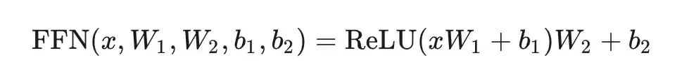
然而,SwiGLU对这一结构进行了优化,将第一层全连接和ReLU激活函数替换为两个权重矩阵和输入的变换,再配合Swish激活函数进行哈达马积操作。
-
swi指的是swish非线性激活函数,
-
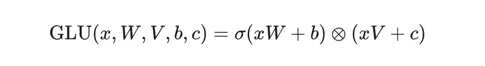
GLU指的是 gated linear unit,输入的向量x分别经过两个linear层,其中一个需要经过非线性激活函数,然后将两者对应元素相乘。

(13696-->5120)((swish(5120-->13696) * (5120-->13696) ))
class SwiGLU(torch.nn.Module):
    def __init__(
        self,
        hidden_size: int,
        intermediate_size: int,
        hidden_act: str,
    ):
        super().__init__()
        self.w1 = torch.nn.Linear(hidden_size, intermediate_size, bias=False) ###(5120*13696)
        self.w2 = torch.nn.Linear(intermediate_size, hidden_size, bias=False) ###(13696*5120)
        self.w3 = torch.nn.Linear(hidden_size, intermediate_size, bias=False)  ###(5120*13696)
        self.act_fn = ACT2FN[hidden_act] ###可以是swish, silu等非线性激活函数

    def forward(self, x):
        return self.w2(self.act_fn(self.w1(x)) * self.w3(x))
        # 或 return self.w2(F.silu(self.w1(x)) * self.w3(x))
KV-Cache
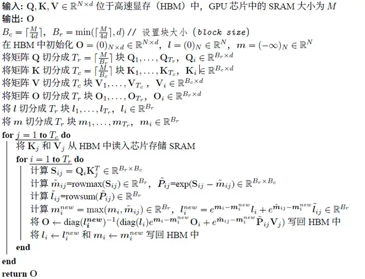
长文本输入的情况下,占用的显存线性随句长增长,此时需要做cache优化,KV-Cache就是用来缓存自回归模型中Attention中的Key和Value的,只出现在Transformer-Decoder中(如GPT/LLAMA中,T5的Decoder中,而BERT就没有),KV-Cache是做LLM模型层面的推理加速,而FlashAttention则是GPU硬件算法优化。

CLM (causal language model) task:
- NTP (next token prediction) training:
Input: [SOS] Love that can quickly seize the gentle heart
Target: Love that can quickly seize the gentle heart [EOS]
- NTP inference
SOS: start of sentence
EOS: end of sentence
| Input | Output | |
|---|---|---|
| t=1 | [SOS] | Love |
| t=2 | [SOS] Love | Love that |
| t=3 | [SOS] Love that | Love that can |
| t=4 | [SOS] Love that can | Love that can quickly |
| t=5 | [SOS] Love that can quickly | Love that can quickly seize |
| t=6 | [SOS] Love that can quickly seize | Love that can quickly seize the |
| t=7 | [SOS] Love that can quickly seize the | Love that can quickly seize the gentle |
| t=8 | [SOS] Love that can quickly seize the gentle | Love that can quickly seize the gentle heart |
| t=9 | [SOS] Love that can quickly seize the gentle heart | Love that can quickly seize the gentle heart [EOS] |

就像上面描述的一样,自回归模型上次的输出,作为本次的输入,历史信息会作为K和V与Q进行Attention运算,但是随着历史信息内容的增加,K和V可能是非常庞大的matrix,而Q还是一个vector。但存在一个问题,每次transformer都会重复推理前面已经有的token,这样会重复执行之前发生过的矩阵运算。

推理时,要预测下个token只需要当前最尾的一个q。我们可以得出一个结论,Q[-1], K[:], V[:]就可以计算next_token!
-
Without KV-Cache, 每次需要计算全Wq(X),Wk(X), Wv(X), 每次需要计算全量Attn。
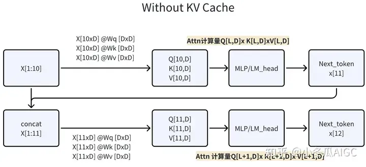
-
With KV-Cache,第一步计算完整Attn,将KV保存成KV_cache。第二步,取第一步的Next Token
计算Q=Wq(
[KV_cache, KV]拼接,计算出QKV。KV-Cache每个循环累增,的memory 量=2*(N层*L长度*D维度)。

使用KV-Cache就是缓存前面已经有的KV的tokens(缓存的是K=Wk@X),减少了X先前已经计算过了token再与Wk相乘。每次只将X中新的token与W计算得到
Attention with KV-Cache源码:不断在max_seq_len维度上append新的KV
class Attention(nn.Module):
    """Multi-head attention module."""
    def __init__(self, args: ModelArgs):

        self.wq = ColumnParallelLinear(args.dim, args.n_heads * self.head_dim)
        self.wk = ColumnParallelLinear(args.dim, self.n_kv_heads * self.head_dim)
        self.wv = ColumnParallelLinear(args.dim, self.n_kv_heads * self.head_dim)
        self.wo = RowParallelLinear(args.n_heads * self.head_dim, args.dim)


        # [8, 1024, 32, 128]
        self.cache_k = torch.zeros(
            (
                args.max_batch_size,    # 8
                args.max_seq_len,       # 1024, 不断地在这个维度上append keys
                self.n_local_kv_heads,  # 32
                self.head_dim,          # 128
            )
        ).cuda()

        #  [8, 1024, 32, 128]
        self.cache_v = torch.zeros(
            (
                args.max_batch_size,    # 8
                args.max_seq_len,       # 1024, 不断地在这个维度上append values
                self.n_local_kv_heads,  # 32
                self.head_dim,          # 128
            )
        ).cuda()

    def forward(
        self,
        x: torch.Tensor,
        start_pos: int,
        freqs_cis: torch.Tensor,
        mask: Optional[torch.Tensor],
    ):
        xq, xk, xv = self.wq(x), self.wk(x), self.wv(x)

        xq = xq.view(bsz, seqlen, self.n_local_heads, self.head_dim)
        xk = xk.view(bsz, seqlen, self.n_local_kv_heads, self.head_dim)
        xv = xv.view(bsz, seqlen, self.n_local_kv_heads, self.head_dim)

        xq, xk = apply_rotary_emb(xq, xk, freqs_cis=freqs_cis)

        self.cache_k = self.cache_k.to(xq)
        self.cache_v = self.cache_v.to(xq)


        self.cache_k[:bsz, start_pos : start_pos + seqlen] = xk
        self.cache_v[:bsz, start_pos : start_pos + seqlen] = xv

        # 这里在复用之前的计算, all_past
        keys = self.cache_k[:bsz, : start_pos + seqlen]
        values = self.cache_v[:bsz, : start_pos + seqlen]

Grouped Query Attention(GQA)
以LLM Foundry 为例,分组查询注意力实现代码如下,与LLM Foundry 中实现的多头自注意力代码相对比,其区别仅在于建立Wqkv 层上:
import torch
import torch.nn as nn
from torch.nn import functional as F
from typing import Optional


class MultiQueryAttention(nn.Module):
    """Multi-Query self attention.
    Using torch or triton attention implemetation enables user to also use
    additive bias.
    """
    def __init__(
        self,
        d_model: int,
        n_heads: int,
        device: Optional[str] = None,
    ):
        super().__init__()
        self.d_model = d_model
        self.n_heads = n_heads
        self.head_dim = d_model // n_heads
        self.Wqkv = nn.Linear( # Multi-Query Attention 创建
            d_model,
            d_model + 2 * self.head_dim, # 只创建查询的头向量,所以只有1 个d_model
            device=device, # 而键和值则共享各自的一个head_dim 的向量
        )
        self.out_proj = nn.Linear(
            self.d_model,
            self.d_model,
            device=device
        )
        self.out_proj._is_residual = True # type: ignore
    def forward(
        self,
        x,
    ):
        qkv = self.Wqkv(x) # (1, 512, 960)
        query, key, value = qkv.split( # query -> (1, 512, 768)
            [self.d_model, self.head_dim, self.head_dim], # key -> (1, 512, 96)
            dim=2 # value -> (1, 512, 96)
        )
        context, attn_weights, past_key_value = F.scaled_dot_product_attention(query, key, value,
            self.n_heads, multiquery=True)
        return self.out_proj(context), attn_weights, past_key_value
LLaMa Finetine——Alpaca、Vicuna
- LLaMa:是
pertrained model,类似text-davini-003(gpt3),训练数据是公开的1T tokens。支持4k context window的长度。 - Self Instruction (SFT):在LLaMa权重基础上进行instruction tuning。(性能:Vicuna>Alpaca>LLaMa)
- Alpaca:prompt和answer都来自ChatGPT,52K samples。
- Vicuna:prompt来自互联网,answer都来自ShareGPT,70K samples;更长的context window;Vicuna weights是基于LLaMa weights的二次权重。
LLaMa LoRA SFT
LoRA全称Low-Rank Adaption of LLM,在不破坏原始参数的基础上(freezed LLM weights),实现对参数
的等价微调,本质是微调1个
Linear Layer参数矩阵的2个低秩矩阵
和
(超参数:低秩的rank=
,SVD分解减少参数量),实现模型的高效微调(PEFT)得到推理时新的参数矩阵
,通常微调的
Linear Layer是Attention的的
,其中
用于控制lora权重的比例:
如d=100,k=500,r=5,对比 和
矩阵的参数量:(5100+5500)/(100*500)=3k/5w=6%,这就叫做Parameter efficiency参数高效的微调!超参数
越小,参数约节省,但微调出来的模型性能也可能越差。
Linear layer的LoRA伪代码:(这部分可以用peft库的get_peft_model实现)
import math
import torch
from torch import nn

input_dim = 768  # in_feature dim
output_dim = 768  # out_feature dim
rank = 8

W = ...  # from pretrained model with shape (input_dim, output_dim)
W_A = nn.Parameter(torch.empty(input_dim, rank))
W_B = nn.Parameter(torch.empty(rank, output_dim))

nn.init.kaiming_uniform_(W_A, a=math.sqrt(5))
nn.init.zeros_(W_B, a=math.sqrt(5))

def lora_forward(self, x, W, W_A, W_B):
    h = x @ W  + alpha * x @ (W_A @ W_B)
    return h
原始llama模型结构:
LlamaForCausalLM(
  (model): LlamaModel(
    (embed_tokens): Embedding(32000, 4096, padding_idx=31999)
    (layers): ModuleList(
      (0-31): 32 x LlamaDecoderLayer(
        (self_attn): LlamaAttention(
          (q_proj): Linear8bitLt(in_features=4096, out_features=4096, bias=False)
          (k_proj): Linear8bitLt(in_features=4096, out_features=4096, bias=False)
          (v_proj): Linear8bitLt(in_features=4096, out_features=4096, bias=False)
          (o_proj): Linear8bitLt(in_features=4096, out_features=4096, bias=False)
          (rotary_emb): LlamaRotaryEmbedding()
        )
        (mlp): LlamaMLP(
          (gate_proj): Linear8bitLt(in_features=4096, out_features=11008, bias=False)
          (down_proj): Linear8bitLt(in_features=11008, out_features=4096, bias=False)
          (up_proj): Linear8bitLt(in_features=4096, out_features=11008, bias=False)
          (act_fn): SiLUActivation()
        )
        (input_layernorm): LlamaRMSNorm()
        (post_attention_layernorm): LlamaRMSNorm()
      )
    )
    (norm): LlamaRMSNorm()
  )
  (lm_head): Linear(in_features=4096, out_features=32000, bias=False)
)
huggingface的trl库有专用于模型指令微调的SFTTrainer,封装度较高,上手难度小,整个微调流程大约分为三步: 1. 模型和tokenizer载入。2. SFT数据准备。3. 模型训练和保存(上传huggingface)。其中device_map="auto"会进行模型并行。
import torch
from datasets import load_dataset
from transformers import (
    AutoModelForCausalLM,
    AutoTokenizer,
    BitsAndBytesConfig,
    TrainingArguments,
    pipeline)
from peft import LoraConfig
from trl import SFTTrainer


# Model and tokenizer names
base_model_name = "/data3/huggingface/LLM/Llama-2-7b-chat-hf"
new_model_name = "llama-2-7b-enhanced" #You can give your own name for fine tuned model
# Tokenizer
llama_tokenizer = AutoTokenizer.from_pretrained(base_model_name, trust_remote_code=True)
llama_tokenizer.pad_token = llama_tokenizer.eos_token
llama_tokenizer.padding_side = "right"
# Model
base_model = AutoModelForCausalLM.from_pretrained(
    base_model_name,
    device_map="auto"
)
base_model.config.use_cache = False
base_model.config.pretraining_tp = 1


# Load Dataset
data_name = "mlabonne/guanaco-llama2-1k"
training_data = load_dataset(data_name, split="train")
# check the data
print(training_data.shape)
# #11 is a QA sample in English
print(training_data[11])


# Training Params
train_params = TrainingArguments(
    output_dir="./results_modified",
    num_train_epochs=1,
    per_device_train_batch_size=4,
    gradient_accumulation_steps=1,
    optim="paged_adamw_32bit",
    save_steps=50,
    logging_steps=50,
    learning_rate=4e-5,
    weight_decay=0.001,
    fp16=False,
    bf16=False,
    max_grad_norm=0.3,
    max_steps=-1,
    warmup_ratio=0.03,
    group_by_length=True,
    lr_scheduler_type="constant",
    report_to="tensorboard"
)

from peft import get_peft_model
# LoRA Config
peft_parameters = LoraConfig(
    lora_alpha=8,
    lora_dropout=0.1,
    r=8,
    bias="none",
    task_type="CAUSAL_LM"
)
model = get_peft_model(base_model, peft_parameters)
model.print_trainable_parameters()

# Trainer with LoRA configuration
fine_tuning = SFTTrainer(
    model=base_model,
    train_dataset=training_data,
    peft_config=peft_parameters,
    dataset_text_field="text",
    tokenizer=llama_tokenizer,
    args=train_params
)

# Training
fine_tuning.train()
# Save Model
fine_tuning.model.save_pretrained(new_model_name)


# Reload model in FP16 and merge it with LoRA weights
base_model = AutoModelForCausalLM.from_pretrained(
    base_model_name,
    low_cpu_mem_usage=True,
    return_dict=True,
    torch_dtype=torch.float16,
    device_map="auto"
)
from peft import LoraConfig, PeftModel
model = PeftModel.from_pretrained(base_model, new_model_name)
model = model.merge_and_unload()

# Reload tokenizer to save it
tokenizer = AutoTokenizer.from_pretrained(base_model_name, trust_remote_code=True)
tokenizer.pad_token = tokenizer.eos_token
tokenizer.padding_side = "right"
from huggingface_hub import login
# You need to use your Hugging Face Access Tokens
login("xxxxxxxxxxxxxxxxxxxxxxxxxxxxxxxxxxxxx")
# Push the model to Hugging Face. This takes minutes and time depends the model size and your
# network speed.
model.push_to_hub(new_model_name, use_temp_dir=False)
tokenizer.push_to_hub(new_model_name, use_temp_dir=False)

# Generate text using base model
query = "What do you think is the most important part of building an AI chatbot?"
text_gen = pipeline(task="text-generation", model=base_model_name, tokenizer=llama_tokenizer, max_length=200)
output = text_gen(f"<s>[INST] {query} [/INST]")
print(output[0]['generated_text'])

# Generate text using fine-tuned model
query = "What do you think is the most important part of building an AI chatbot?"
text_gen = pipeline(task="text-generation", model=new_model_name, tokenizer=llama_tokenizer, max_length=200)
output = text_gen(f"<s>[INST] {query} [/INST]")
print(output[0]['generated_text'])
Alpaca inference
Alpaca-lora-7b :基于LLaMA-7b 在 Stanford Alpaca dataset上进行LoRA微调得到。下面config中的Lora target modules就是指q_proj、k_proj、v_proj、o_proj中会包含lora_A和lora_B。Lora rank=16。
Epochs: 10 (load from best epoch)
Batch size: 128
Cutoff length: 512
Learning rate: 3e-4
Lora r: 16
Lora target modules: q_proj, k_proj, v_proj, o_proj
4bit或8bit推理:使用 4 比特量化的不同变体,例如 NF4 (NormalFloat4 (默认) ) 或纯 FP4 量化。从理论分析和实证结果来看,我们建议使用 NF4 量化以获得更好的性能。其他选项包括 bnb_4bit_use_double_quant ,它在第一轮量化之后会进行第二轮量化,为每个参数额外节省 0.4 比特。最后是计算类型,虽然 4 比特 bitsandbytes 以 4 比特存储权重,但计算仍然以 16 或 32 比特进行,这里可以选择任意组合 (float16、bfloat16、float32 等)。如果使用 16 比特计算数据类型 (默认 torch.float32),矩阵乘法和训练将会更快。用户应该利用 transformers 中最新的 BitsAndBytesConfig 来更改这些参数。下面是使用 NF4 量化加载 4 比特模型的示例,例子中使用了双量化以及 bfloat16 计算数据类型以加速训练。
import torch
import transformers
from transformers import LlamaTokenizer, LlamaForCausalLM, GenerationConfig, BitsAndBytesConfig

# BitsAndBytesConfig设置推理精度
nf4_config = BitsAndBytesConfig(
   load_in_4bit=True,
   bnb_4bit_quant_type="nf4",
   bnb_4bit_use_double_quant=True,
   bnb_4bit_compute_dtype=torch.bfloat16
)

# load base_model and tokenizer
model = LlamaForCausalLM.from_pretrained("/data3/huggingface/LLM/Llama-2-7b-chat-hf", quantization_config=nf4_config, device_map="auto")
tokenizer = LlamaTokenizer.from_pretrained("/data3/huggingface/LLM/Llama-2-7b-chat-hf")
# load lora using peft
from peft import PeftModel
model = PeftModel.from_pretrained(model, "/data3/huggingface/LLM/alpaca-lora-7b")


from peft import mapping
from peft.utils import other
print('model_type', model.config.model_type)
print(model.peft_config['default'].target_modules)
#默认的 target module
print(other.TRANSFORMERS_MODELS_TO_LORA_TARGET_MODULES_MAPPING)


def generate_prompt(instruction, input=None):
    if input:
        return f"""Below is an instruction that describes a task, paired with an input that provides further context. Write a response that appropriately completes the request.

### Instruction:
{instruction}

### Input:
{input}

### Response:"""
    else:
        return f"""Below is an instruction that describes a task. Write a response that appropriately completes the request.

### Instruction:
{instruction}

### Response:"""

generation_config = GenerationConfig(
    temperature=1.5,
    # nucleus sampling
    top_p=0.8,
    num_beams=4,
)

def inference(instruction, input=None):
    prompt = generate_prompt(instruction, input)
#     print(prompt)
    inputs = tokenizer(prompt, return_tensors="pt")
    input_ids = inputs["input_ids"].cuda()
    generation_output = model.generate(
        input_ids=input_ids,
        generation_config=generation_config,
        return_dict_in_generate=True,
        output_scores=True,
        max_new_tokens=256
    )
    for s in generation_output.sequences:
        output = tokenizer.decode(s)
        print("Response:", output.split("### Response:")[1].strip())


inference(input("Instruction: "))
加载lora后的模型结构:可以看到q_proj、k_proj、v_proj、o_proj中会包含lora_A和lora_B。
PeftModelForCausalLM(
  (base_model): LoraModel(
    (model): LlamaForCausalLM(
      (model): LlamaModel(
        (embed_tokens): Embedding(32000, 4096, padding_idx=31999)
        (layers): ModuleList(
          (0-31): 32 x LlamaDecoderLayer(
            (self_attn): LlamaAttention(
              (q_proj): Linear8bitLt(
                in_features=4096, out_features=4096, bias=False
                (lora_dropout): ModuleDict(
                  (default): Dropout(p=0.05, inplace=False)
                )
                (lora_A): ModuleDict(
                  (default): Linear(in_features=4096, out_features=16, bias=False)
                )
                (lora_B): ModuleDict(
                  (default): Linear(in_features=16, out_features=4096, bias=False)
                )
                (lora_embedding_A): ParameterDict()
                (lora_embedding_B): ParameterDict()
              )
              (k_proj): Linear8bitLt(
                in_features=4096, out_features=4096, bias=False
                (lora_dropout): ModuleDict(
                  (default): Dropout(p=0.05, inplace=False)
                )
                (lora_A): ModuleDict(
                  (default): Linear(in_features=4096, out_features=16, bias=False)
                )
                (lora_B): ModuleDict(
                  (default): Linear(in_features=16, out_features=4096, bias=False)
                )
                (lora_embedding_A): ParameterDict()
                (lora_embedding_B): ParameterDict()
              )
              (v_proj): Linear8bitLt(
                in_features=4096, out_features=4096, bias=False
                (lora_dropout): ModuleDict(
                  (default): Dropout(p=0.05, inplace=False)
                )
                (lora_A): ModuleDict(
                  (default): Linear(in_features=4096, out_features=16, bias=False)
                )
                (lora_B): ModuleDict(
                  (default): Linear(in_features=16, out_features=4096, bias=False)
                )
                (lora_embedding_A): ParameterDict()
                (lora_embedding_B): ParameterDict()
              )
              (o_proj): Linear8bitLt(
                in_features=4096, out_features=4096, bias=False
                (lora_dropout): ModuleDict(
                  (default): Dropout(p=0.05, inplace=False)
                )
                (lora_A): ModuleDict(
                  (default): Linear(in_features=4096, out_features=16, bias=False)
                )
                (lora_B): ModuleDict(
                  (default): Linear(in_features=16, out_features=4096, bias=False)
                )
                (lora_embedding_A): ParameterDict()
                (lora_embedding_B): ParameterDict()
              )
              (rotary_emb): LlamaRotaryEmbedding()
            )
            (mlp): LlamaMLP(
              (gate_proj): Linear8bitLt(in_features=4096, out_features=11008, bias=False)
              (down_proj): Linear8bitLt(in_features=11008, out_features=4096, bias=False)
              (up_proj): Linear8bitLt(in_features=4096, out_features=11008, bias=False)
              (act_fn): SiLUActivation()
            )
            (input_layernorm): LlamaRMSNorm()
            (post_attention_layernorm): LlamaRMSNorm()
          )
        )
        (norm): LlamaRMSNorm()
      )
      (lm_head): Linear(in_features=4096, out_features=32000, bias=False)
    )
  )
)
版权声明:本文为博主作者:Yuezero_原创文章,版权归属原作者,如果侵权,请联系我们删除!
原文链接:https://blog.csdn.net/weixin_54338498/article/details/135269411