文章目录
- 1 引言
- 2 卷积神经网络概述
- 2.1 卷积神经网络的背景介绍
- 2.2 CNN的网络结构
- 2.2.1 卷积层
- 2.2.2 激活函数
- 2.2.3 池化层
- 2.2.4 全连接层
- 2.3 CNN的训练过程图解
- 2.4 CNN的基本特征
- 2.4.1 局部感知(Local Connectivity)
- 2.4.2 参数共享(Parameter Sharing)
- 3 数据集介绍
- 4 猫狗识别(tensorflow)
- 4.1 搭建卷积神经网络模型
- 4.2 训练模型
- 4.3 识别预测结果
- 5 猫狗分类(keras基准模型)
- 5.1 构建网络模型
- 5.2 训练配置
- 5.3 模型训练
- 5.4 结果可视化
- 6 基准模型的调整
- 6.1 图像增强
- 6.2 添加一层dropout
- 6.3 训练模型
- 总结
1 引言
很巧,笔者在几月前的计算机设计大赛作品设计中也采用了猫狗识别,目前已推国赛评选中
但当时所使用的方法与本次作业要求不太一致,又重新做了一遍,下文将以本次作业要求为主,介绍CNN卷积神经网络实现猫狗识别
猫狗识别和狗品种识别是计算机视觉领域中一个重要且具有挑战性的问题。在猫狗识别问题中,我们需要将图像中的猫和狗进行分类。而在狗品种识别问题中,我们需要识别出不同品种的狗,例如哈士奇、金毛等。这些问题在现实生活中具有广泛的应用,如动物保护、智能监控等领域。下图为我个人搜集的我国宠物行业现状部分图表。

2 卷积神经网络概述
2.1 卷积神经网络的背景介绍
卷积神经网络(Convolutional Neural Networks,简称CNN)是一种具有局部连接、权值共享等特点的深层前馈神经网络(Feedforward Neural Networks),是深度学习(deep learning)的代表算法之一,擅长处理图像特别是图像识别等相关机器学习问题,比如图像分类、目标检测、图像分割等各种视觉任务中都有显著的提升效果,是目前应用最广泛的模型之一。
卷积神经网络具有表征学习(representation learning)能力,能够按其阶层结构对输入信息进行平移不变分类(shift-invariant classification),可以进行监督学习和非监督学习,其隐含层内的卷积核参数共享和层间连接的稀疏性使得卷积神经网络能够以较小的计算量对格点化(grid-like topology)特征,例如像素和音频进行学习、有稳定的效果且对数据没有额外的特征工程(feature engineering)要求,并被大量应用于计算机视觉、自然语言处理等领域。
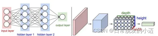
图中左为神经网络(全连接结构),右为卷积神经网络。
2.2 CNN的网络结构
CNN的网络结构图如下:
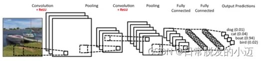
卷积神经网络的基本结构大致包括:卷积层、激活函数、池化层、全连接层、输出层等。
2.2.1 卷积层
卷积层是卷积神经网络最重要的一个层次,也是“卷积神经网络”的名字来源。卷积神经网路中每层卷积层由若干卷积单元组成,每个卷积单元的参数都是通过反向传播算法优化得到的。
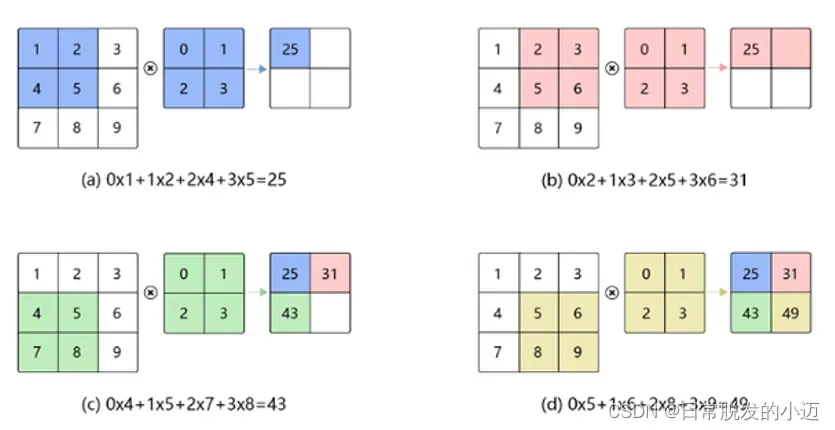
卷积操作图解如下:
在这个卷积层,有两个关键操作:
- 局部关联。每个神经元看做一个滤波器(filter)。
- 窗口(receptive field)滑动, filter对局部数据计算。
卷积运算的目的是提取输入的不同特征,某些卷积层可能只能提取一些低级的特征如边缘、线条和角等层级,更多层的网路能从低级特征中迭代提取更复杂的特征。
卷积层的作用是对输入数据进行卷积操作,也可以理解为滤波过程,一个卷积核就是一个窗口滤波器,在网络训练过程中,使用自定义大小的卷积核作为一个滑动窗口对输入数据进行卷积。
卷积过程实质上就是两个矩阵做乘法,在卷积过程后,原始输入矩阵会有一定程度的缩小,比如自定义卷积核大小为3*3,步长为1时,矩阵长宽会缩小2,所以在一些应用场合下,为了保持输入矩阵的大小,我们在卷积操作前需要对数据进行扩充,常见的扩充方法为0填充方式。
卷积层中还有两个重要的参数,分别是偏置和激活(独立层,但一般将激活层和卷积层放在一块)。
偏置向量的作用是对卷积后的数据进行简单线性的加法,就是卷积后的数据加上偏置向量中的数据,然后为了增加网络的一个非线性能力,需要对数据进行激活操作,在神经元中,就是将没有的数据率除掉,而有用的数据则可以输入神经元,让人做出反应。
2.2.2 激活函数
最常用的激活函数目前有Relu、tanh、sigmoid,着重介绍一下Relu函数(即线性整流层(Rectified Linear Units layer, 简称ReLU layer)),Relu函数是一个线性函数,它对负数取0,正数则为y=x(即输入等于输出),即f(x)=max(0,x),它的特点是收敛快,求梯度简单,但较脆弱。
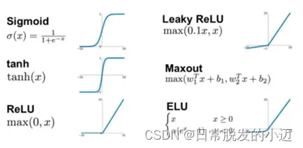
由于经过Relu函数激活后的数据0值一下都变成0,而这部分数据难免有一些我们需要的数据被强制取消,所以为了尽可能的降低损失,我们就在激活层的前面,卷积层的后面加上一个偏置向量,对数据进行一次简单的线性加法,使得数据的值产生一个横向的偏移,避免被激活函数过滤掉更多的信息。
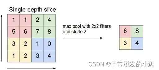
2.2.3 池化层
池化层通常在卷积层之后会得到维度很大的特征,将特征切成几个区域,取其最大值或平均值,得到新的、维度较小的特征。
池化方式一般有两种,一种为取最大值,另一种为取均值,池化的过程也是一个移动窗口在输入矩阵上滑动,滑动过程中去这个窗口中数据矩阵上最大值或均值作为输出,池化层的大小一般为2*2,步长为1。
池化层的具体作用:
- 特征不变性,也就是我们在图像处理中经常提到的特征的尺度不变性,池化操作就是图像的resize,平时一张狗的图像被缩小了一倍我们还能认出这是一张狗的照片,这说明这张图像中仍保留着狗最重要的特征,我们一看就能判断图像中画的是一只狗,图像压缩时去掉的信息只是一些无关紧要的信息,而留下的信息则是具有尺度不变性的特征,是最能表达图像的特征。
- 特征降维,我们知道一幅图像含有的信息是很大的,特征也很多,但是有些信息对于我们做图像任务时没有太多用途或者有重复,我们可以把这类冗余信息去除,把最重要的特征抽取出来,这也是池化操作的一大作用。
- 在一定程度上防止过拟合,更方便优化。
2.2.4 全连接层
全连接层往往在分类问题中用作网络的最后层,作用主要为将数据矩阵进行全连接,然后按照分类数量输出数据,在回归问题中,全连接层则可以省略,但是我们需要增加卷积层来对数据进行逆卷积操作。
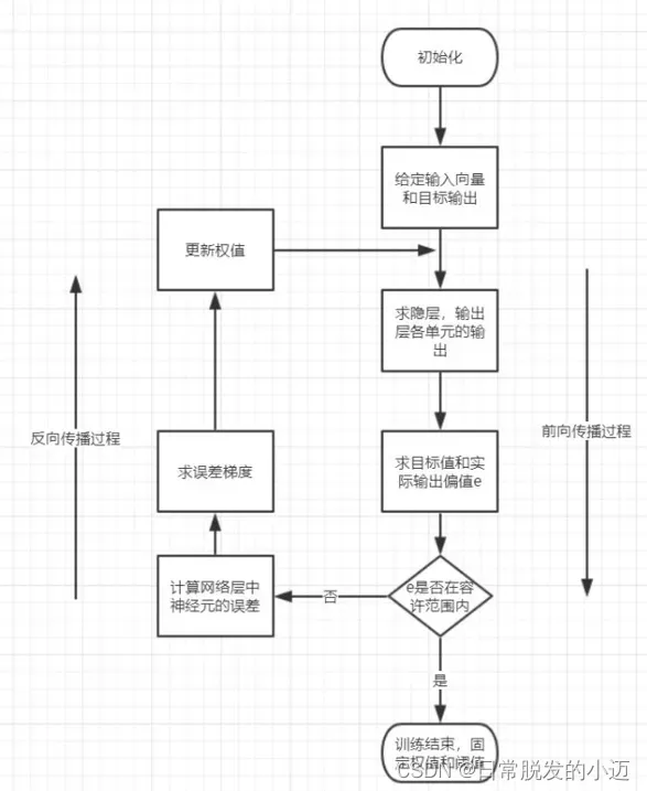
2.3 CNN的训练过程图解
-
前向传播阶段:
选取训练样本(x,y),将x输入网络中。随机初始化权值(一般情况下选取小数),信息从输入层经过一层一层的特征提取和转换,最后到达输出层,得到输出结果。 -
反向传播阶段:
输出结果与理想结果对比,计算全局性误差(即Loss)。得到的误差反向传递给不同层的神经元,按照“迭代法”调整权值和偏重,寻找全局性最优的结果。
2.4 CNN的基本特征
2.4.1 局部感知(Local Connectivity)
卷积层解决这类问题的一种简单方法是对隐含单元和输入单元间的连接加以限制:每个隐含单元仅仅只能连接输入单元的一部分。例如,每个隐含单元仅仅连接输入图像的一小片相邻区域。
2.4.2 参数共享(Parameter Sharing)
在卷积层中每个神经元连接数据窗的权重是固定的,每个神经元只关注一个特性。神经元就是图像处理中的滤波器,比如边缘检测专用的Sobel滤波器,即卷积层的每个滤波器都会有自己所关注一个图像特征,比如垂直边缘,水平边缘,颜色,纹理等等,这些所有神经元加起来就好比就是整张图像的特征提取器集合。
权值共享使得我们能更有效的进行特征抽取,因为它极大的减少了需要学习的自由变量的个数。通过控制模型的规模,卷积网络对视觉问题可以具有很好的泛化能力。
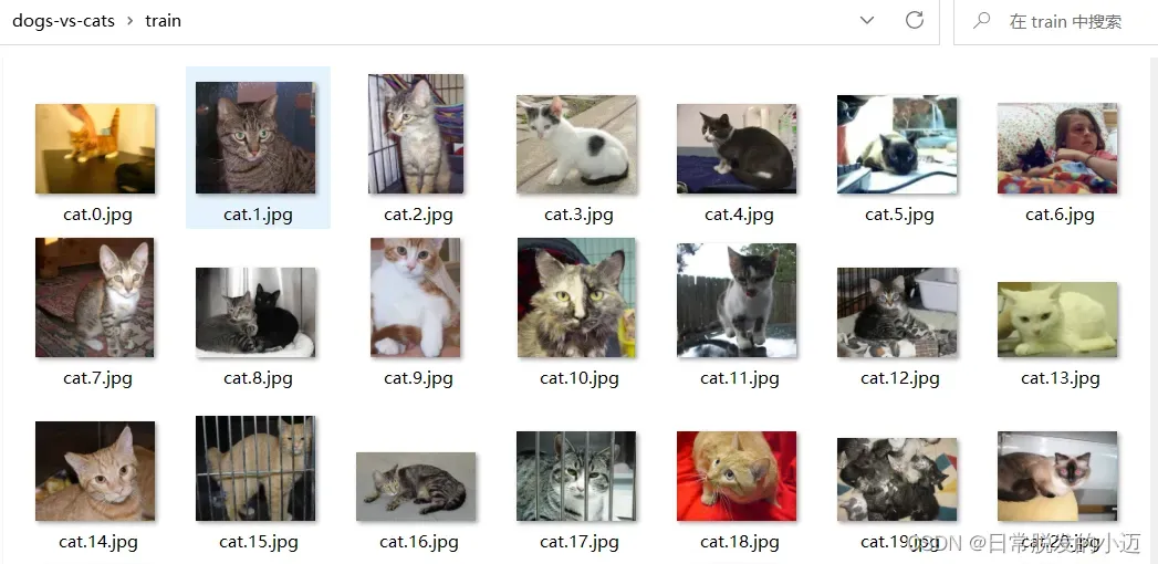
3 数据集介绍
本次实验采用的是kaggle猫狗识别数据集,共包含了25000张JPEG数据集照片,其中猫和狗的照片各占12500张。数据集大小经过压缩打包后占543MB。
官网下载链接如下:
https://www.kaggle.com/c/dogs-vs-cats/data
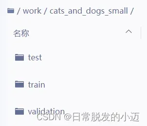
由于数据集数量过于大,对于一个小作业的测试来说,所以要在下载的kaggle数据集基础上,创建一个新的小数据集,其中包含三个子集。
即猫和狗的数据集:各 1000 个样本的训练集、各 500 个样本的验证集、各 500 个样本的测试集。
创建新的小数据集
生成各个文件夹路径,并将对应的训练集、验证集、测试集复制进去生成新的小数据集。
import os, shutil
# 下载的kaggle数据集路径
original_dataset_dir = 'data/train'
# 新的小数据集放置路径
base_dir = 'work/cats_and_dogs_small'
os.mkdir(base_dir)
train_dir = os.path.join(base_dir, 'train')
os.mkdir(train_dir)
validation_dir = os.path.join(base_dir, 'validation')
os.mkdir(validation_dir)
test_dir = os.path.join(base_dir, 'test')
os.mkdir(test_dir)

train_cats_dir = os.path.join(train_dir, 'cats')
os.mkdir(train_cats_dir)
train_dogs_dir = os.path.join(train_dir, 'dogs')
os.mkdir(train_dogs_dir)
validation_cats_dir = os.path.join(validation_dir, 'cats')
os.mkdir(validation_cats_dir)
validation_dogs_dir = os.path.join(validation_dir, 'dogs')
os.mkdir(validation_dogs_dir)
test_cats_dir = os.path.join(test_dir, 'cats')
os.mkdir(test_cats_dir)
test_dogs_dir = os.path.join(test_dir, 'dogs')
os.mkdir(test_dogs_dir)

fnames = ['cat.{}.jpg'.format(i) for i in range(1000)]
for fname in fnames:
    src = os.path.join(original_dataset_dir, fname)
    dst = os.path.join(train_cats_dir, fname)
    shutil.copyfile(src, dst)

fnames = ['cat.{}.jpg'.format(i) for i in range(1000, 1500)]
for fname in fnames:
    src = os.path.join(original_dataset_dir, fname)
    dst = os.path.join(validation_cats_dir, fname)
    shutil.copyfile(src, dst)

fnames = ['cat.{}.jpg'.format(i) for i in range(1500, 2000)]
for fname in fnames:
     src = os.path.join(original_dataset_dir, fname)
     dst = os.path.join(test_cats_dir, fname)
     shutil.copyfile(src, dst)

fnames = ['dog.{}.jpg'.format(i) for i in range(1000)]
for fname in fnames:
    src = os.path.join(original_dataset_dir, fname)
    dst = os.path.join(train_dogs_dir, fname)
    shutil.copyfile(src, dst)

fnames = ['dog.{}.jpg'.format(i) for i in range(1000, 1500)]
for fname in fnames:
    src = os.path.join(original_dataset_dir, fname)
    dst = os.path.join(validation_dogs_dir, fname)
    shutil.copyfile(src, dst)

fnames = ['dog.{}.jpg'.format(i) for i in range(1500, 2000)]
for fname in fnames:
    src = os.path.join(original_dataset_dir, fname)
    dst = os.path.join(test_dogs_dir, fname)
    shutil.copyfile(src, dst)

print('total training cat images:', len(os.listdir(train_cats_dir)))
print('total training dog images:', len(os.listdir(train_dogs_dir)))
print('total validation cat images:', len(os.listdir(validation_cats_dir)))
print('total validation dog images:', len(os.listdir(validation_dogs_dir)))
print('total test cat images:', len(os.listdir(test_cats_dir)))
print('total test dog images:', len(os.listdir(test_dogs_dir)))
上述程序输出结果为:
total training cat images: 1000
total training dog images: 1000
total validation cat images: 500
total validation dog images: 500
total test cat images: 500
total test dog images: 500
分好后的数据集目录结构如下:
4 猫狗识别(tensorflow)
4.1 搭建卷积神经网络模型
创建一个新的python程序并导入相关numpy、tensorflow等基础科学软件包
import tensorflow as tf
import numpy as np
import tensorflow.contrib.slim as slim
from PIL import Image,ImageFont, ImageDraw
创建大量的权重和偏置项,进行卷积和池化。定义一个解析输入参数的函数,代码如下:
def build_graph(top_k):
    # 调用tf.placeholder函数操作,定义传入图表中的shape参数,后续还会将实际的训练用例传入图表。在训练循环(train_op)的后续步骤中,传入的整个图像和标签数据集会被切片,以符合每一个操作所设置的shape参数值,占位符操作将会填补以符合这个shape参数值。然后使用feed_dict参数,将数据传入sess1.run()函数。
    keep_prob = tf.placeholder(dtype=tf.float32, shape=[], name='keep_prob')
    images = tf.placeholder(dtype=tf.float32, shape=[None, 64, 64, 3], name='image_batch')
    labels = tf.placeholder(dtype=tf.int64, shape=[None], name='label_batch')

    # 定义卷积,传入x和参数,slim..conv2d(input, filter, strides, padding, use_cudnn_on_gpu=None, name=None)
    conv_1 = slim.conv2d(images, 64, [3, 3], 3, padding='SAME', scope='conv1')
    # 定义池化,传入x, pooling, slim..max_pool(value, ksize, strides, padding, name=None)
    max_pool_1 = slim.max_pool2d(conv_1, [2, 2], [2, 2], padding='SAME')
    conv_2 = slim.conv2d(max_pool_1, 128, [3, 3], padding='SAME', scope='conv2')
    max_pool_2 = slim.max_pool2d(conv_2, [2, 2], [2, 2], padding='SAME')
    conv_3 = slim.conv2d(max_pool_2, 256, [3, 3], padding='SAME', scope='conv3')
    max_pool_3 = slim.max_pool2d(conv_3, [2, 2], [2, 2], padding='SAME')

    conv_4 = slim.conv2d(max_pool_3, 512, [3, 3], padding='SAME', scope='conv4')
    conv_5 = slim.conv2d(conv_4, 512, [3, 3], padding='SAME', scope='conv5')
    max_pool_4 = slim.max_pool2d(conv_5, [2, 2], [2, 2], padding='SAME')

    flatten = slim.flatten(max_pool_4)

    fc1 = slim.fully_connected(slim.dropout(flatten, keep_prob), 1024, activation_fn=tf.nn.tanh, scope='fc1')
    logits = slim.fully_connected(slim.dropout(fc1, keep_prob), 2, activation_fn=None, scope='fc2')
    # loss()函数通过添加所需的损失操作,进一步构建图表。
    loss = tf.reduce_mean(tf.nn.sparse_softmax_cross_entropy_with_logits(logits=logits, labels=labels))
    accuracy = tf.reduce_mean(tf.cast(tf.equal(tf.argmax(logits, 1), labels), tf.float32))
    global_step = tf.get_variable("step", [], initializer=tf.constant_initializer(0.0), trainable=False)
    rate = tf.train.exponential_decay(2e-4, global_step, decay_steps=2000, decay_rate=0.97, staircase=True)
    train_op = tf.train.AdamOptimizer(learning_rate=rate).minimize(loss, global_step=global_step)
    probabilities = tf.nn.softmax(logits)
    tf.summary.scalar('loss', loss)
    tf.summary.scalar('accuracy', accuracy)
    merged_summary_op = tf.summary.merge_all()
    predicted_val_top_k, predicted_index_top_k = tf.nn.top_k(probabilities, k=top_k)
    accuracy_in_top_k = tf.reduce_mean(tf.cast(tf.nn.in_top_k(probabilities, labels, top_k), tf.float32))

    return {'images': images,
            'labels': labels,
            'keep_prob': keep_prob,
            'top_k': top_k,
            'global_step': global_step,
            'train_op': train_op,
            'loss': loss,
            'accuracy': accuracy,
            'accuracy_top_k': accuracy_in_top_k,
            'merged_summary_op': merged_summary_op,
            'predicted_distribution': probabilities,
            'predicted_index_top_k': predicted_index_top_k,
            'predicted_val_top_k': predicted_val_top_k}
4.2 训练模型
#!/usr/bin/env python
# -*- coding: utf-8 -*-

"""
---------------------------------------------------------
    Name:       train
    Author:     欧阳紫樱
    Date:       2023-07-02
    Time:       10:48
---------------------------------------------------------
    Software:
                PyCharm
"""

import tensorflow.contrib.slim as slim
import matplotlib.pyplot as plt
import tensorflow as tf
import random
import os
# x = [] --- 初始化存放步数的列表
# y_1 = [] --- 初始化步存准确率的列表
# y_2 = [] --- 初始化存放loss的列表
x = []
y_1 = []
y_2 = []
# class DataIterator: --- 数据迭代器
# __init__()方法是所谓的对象的“构造函数”。self是指向该对象本身的一个引用。self代表实例。
class DataIterator:
    def __init__(self, data_dir):
        # Set FLAGS.charset_size to a small value if available computation power is limited.
        # 如果可用计算能力有限,请将FLAGS.charset_size设置为较小的值。
        # 选择的第一个`charset_size`字符来进行实验
        # Python 文件 truncate() 方法用于截断文件并返回截断的字节长度。
        # 指定长度的话,就从文件的开头开始截断指定长度,其余内容删除;
        # 不指定长度的话,就从文件开头开始截断到当前位置,其余内容删除
        truncate_path = data_dir + ('%05d' % 2)
        print(truncate_path)
        self.image_names = []
        # root为根目录。sub_folder为子文件夹。
        # os.walk() 方法是一个简单易用的文件、目录遍历器。data_dir---数据目录。
        # os.walk() 只产生文件路径。os.path.walk() 产生目录树下的目录路径和文件路径。
        # self.image_names += [os.path.join(root, file_path) for file_path in file_list]
        # os.path.join(root,file_path) 根目录与文件路径组合,形成绝对路径。
        # random.shuffle(self.image_names) --- 将序列的所有元素随机排序,返回随机排序后的序列。
              for root, sub_folder, file_list in os.walk(data_dir):
            if root < truncate_path:
                self.image_names = self.image_names+[os.path.join(root, file_path) for file_path in file_list]
                print(self.image_names)
        random.shuffle(self.image_names)
        # 遍历 --- os.sep 使得写的代码可以跨操作系统
        # split() 通过指定分隔符对字符串进行切片,如果参数 num 有指定值,则仅分隔 num 个子字符串。 返回分割后的字符串列表。
        self.labels = [int(file_name[len(data_dir):].split(os.sep)[0]) for file_name in self.image_names]
        print(self.labels)
    # @property --- 属性
    # len() 方法返回对象(字符、列表、元组等)长度或项目个数
      @property
    def size(self):
        return len(self.labels)
    # @staticmethod --- 静态方法
    # 人工增加训练集的大小. 通过加噪声等方法从已有数据中创造出一批"新"的数据.也就是Data Augmentation
    # tf.image.random_brightness(images, max_delta=0.3) --- 随机改变亮度
    # tf.image.random_contrast(images, 0.8, 1.2) --- 随机改变对比度
       @staticmethod
    def data_augmentation(images):
        images = tf.image.random_brightness(images, max_delta=0.3)
        images = tf.image.random_contrast(images, 0.8, 1.2)
        return images
    # batch_size --- 批尺寸    num_epochs --- 指把所有训练数据完整的过一遍的波数   aug --- 是否增大
    # tf.convert_to_tensor 将给定值转换为张量
    # tf.train.slice_input_producer 在tensor_list中生成一个张量片段。
    # num_epochs:一个整数(可选)。如果指定,slice_input_producer 在生成之前产生每个片段num_epochs次
    # tf.read_file 读取并输出输入文件名的全部内容。
    # tf.image.convert_image_dtype 将图像转换为dtype,并根据需要缩放其值。
    # tf.image.decode_png将PNG编码的图像解码为uint8或uint16张量。channels:解码图像的颜色通道数量为1。images_content:字符串类型的张量。0-d。 PNG编码的图像。
    # tf.image.resize_images使用指定的方法将图像调整为大小。
    # tf.train.shuffle_batch 通过随机混洗张量来创建批次。
    # [images, labels]要排队的张量或词典。batch_size:从队列中提取的新批量大小。
    # capacity:队列中元素的最大数量。min_after_dequeue出队后队列中的最小数量元素,用于确保元素的混合级别。
    def input_pipeline(self, batch_size, num_epochs=None, aug=False):
        images_tensor = tf.convert_to_tensor(self.image_names, dtype=tf.string)
        labels_tensor = tf.convert_to_tensor(self.labels, dtype=tf.int64)
        input_queue = tf.train.slice_input_producer([images_tensor, labels_tensor], num_epochs=num_epochs)
        labels = input_queue[1]
        images_content = tf.read_file(input_queue[0])
        images = tf.image.convert_image_dtype(tf.image.decode_png(images_content, channels=3), tf.float32)
        if aug:
            images = self.data_augmentation(images)
        new_size = tf.constant([64, 64], dtype=tf.int32)
        images = tf.image.resize_images(images, new_size)
        image_batch, label_batch = tf.train.shuffle_batch([images, labels], batch_size=batch_size, capacity=5000,min_after_dequeue=1000)
        return image_batch, label_batch
# 搭建神经网络
# tf.placeholder --- 设置一个容器,用于接下来存放数据
# keep_prob --- dropout的概率,也就是在训练的时候有多少比例的神经元之间的联系断开
# images --- 喂入神经网络的图像,labels --- 喂入神经网络图像的标签
# slim.conv2d --- 卷积层 --- (images, 64, [3, 3], 1, padding='SAME', scope='conv3_1')
# 第一个参数表示输入的训练图像,第二个参数表示滤波器的个数,原来的数据是宽64高64维度1,处理后的数据是维度64,
# 第三个参数是滤波器的大小,宽3高3的矩形,第四个参数是表示输入的维度,第五个参数padding表示加边的方式,第六个参数表示层的名称
# slim.max_pool2d --- 表示池化层 --- 池化就是减小卷积神经网络提取的特征,将比较明显的特征提取了,不明显的特征就略掉
# slim.flatten(max_pool_4) --- 表示将数据压缩
# slim.fully_connected --- 全连接层 --- 也就是一个个的神经元
# slim.dropout(flatten, keep_prob) --- dropout层,在训练的时候随机的断掉神经元之间的连接,keep_prob就是断掉的比例
# tf.reduce_mean --- 得到平均值
# tf.nn.sparse_softmax_cross_entropy_with_logits --- 求得交叉熵
# tf.argmax(logits, 1) --- 得到较大的值
# tf.equal() --- 两个数据相等为True,不等为False --- 用于得到预测准确的个数
# tf.cast() --- 将True和False转为1和0,
# global_step --- 训练的步数 --- initializer=tf.constant_initializer(0.0) --- 步数初始化
# tf.train.AdamOptimizer(learning_rate=0.1) --- 优化器的选择,这个训练使用的Adam优化器
# learning_rate=0.1 --- 学习率 --- 训练的过程也就是神经网络学习的过程
# tf.nn.softmax(logits) --- 得到可能性
# tf.summary.scalar / merged_summary_op --- 用于显示训练过程的数据
# predicted_val_top_k --- 喂入图像得到的可能性,也就是识别得到是哪一个汉字的可能性,top_k表示可能性最大的K个数据
# predicted_index_top_k --- 这个表示识别最大K个可能性汉字的索引 --- 也就是汉字对应的数字
# return 表示这个函数的返回值
def build_graph(top_k):
    keep_prob = tf.placeholder(dtype=tf.float32, shape=[], name='keep_prob')
    images = tf.placeholder(dtype=tf.float32, shape=[None, 64, 64, 3], name='image_batch')
    labels = tf.placeholder(dtype=tf.int64, shape=[None], name='label_batch')
    conv_1 = slim.conv2d(images, 64, [3, 3], 3, padding='SAME', scope='conv1')
    max_pool_1 = slim.max_pool2d(conv_1, [2, 2], [2, 2], padding='SAME')
    conv_2 = slim.conv2d(max_pool_1, 128, [3, 3], padding='SAME', scope='conv2')
    max_pool_2 = slim.max_pool2d(conv_2, [2, 2], [2, 2], padding='SAME')
    conv_3 = slim.conv2d(max_pool_2, 256, [3, 3], padding='SAME', scope='conv3')
    max_pool_3 = slim.max_pool2d(conv_3, [2, 2], [2, 2], padding='SAME')

    conv_4 = slim.conv2d(max_pool_3, 512, [3, 3], padding='SAME', scope='conv4')
    conv_5 = slim.conv2d(conv_4, 512, [3, 3], padding='SAME', scope='conv5')
    max_pool_4 = slim.max_pool2d(conv_5, [2, 2], [2, 2], padding='SAME')

    flatten = slim.flatten(max_pool_4)

    fc1 = slim.fully_connected(slim.dropout(flatten, keep_prob), 1024, activation_fn=tf.nn.tanh, scope='fc1')
    logits = slim.fully_connected(slim.dropout(fc1, keep_prob), 2, activation_fn=None, scope='fc2')
    loss = tf.reduce_mean(tf.nn.sparse_softmax_cross_entropy_with_logits(logits=logits, labels=labels))
    accuracy = tf.reduce_mean(tf.cast(tf.equal(tf.argmax(logits, 1), labels), tf.float32))
    global_step = tf.get_variable("step", [], initializer=tf.constant_initializer(0.0), trainable=False)
    rate = tf.train.exponential_decay(2e-4, global_step, decay_steps=2000, decay_rate=0.97, staircase=True)
    train_op = tf.train.AdamOptimizer(learning_rate=rate).minimize(loss, global_step=global_step)
    probabilities = tf.nn.softmax(logits)
    tf.summary.scalar('loss', loss)
    tf.summary.scalar('accuracy', accuracy)
    merged_summary_op = tf.summary.merge_all()
    predicted_val_top_k, predicted_index_top_k = tf.nn.top_k(probabilities, k=top_k)
    accuracy_in_top_k = tf.reduce_mean(tf.cast(tf.nn.in_top_k(probabilities, labels, top_k), tf.float32))

    return {'images': images,
            'labels': labels,
            'keep_prob': keep_prob,
            'top_k': top_k,
            'global_step': global_step,
            'train_op': train_op,
            'loss': loss,
            'accuracy': accuracy,
            'accuracy_top_k': accuracy_in_top_k,
            'merged_summary_op': merged_summary_op,
            'predicted_distribution': probabilities,
            'predicted_index_top_k': predicted_index_top_k,
            'predicted_val_top_k': predicted_val_top_k}
# def train(): --- 训练神经网络
# DataIterator(data_dir='./data/train/') --- 调用函数 --- 得到训练数据集
# DataIterator(data_dir='./data/test/') --- 调用函数 --- 得到测试数据集
# with tf.Session() as sess: --- 新建一个会话
# train_feeder.input_pipeline(batch_size=128, aug=True) --- 得到训练数据集和训练数据集标签
# test_feeder.input_pipeline(batch_size=128) --- 得到测试数据集和测试数据集标签, 个数为128
# build_graph(top_k=1) --- 声明一个网络,参数为1,
# sess.run(tf.global_variables_initializer()) --- 初始化全部的参数
# tf.train.Coordinator() --- 线程的协调者。这个类实现了一个简单的机制来协调一组线程的终止。
# tf.train.start_queue_runners(sess=sess, coord=coord) --- 开始在图表中收集的所有队列运行者。为图中收集的所有队列运行者启动线程。
# coord:可选协调器,用于协调启动的线程
# tf.train.Saver() --- 保存并恢复变量
def train():
    train_feeder = DataIterator(data_dir='./data/train/')
    test_feeder = DataIterator(data_dir='./data/test/')

    with tf.Session() as sess:
        train_images, train_labels = train_feeder.input_pipeline(batch_size=28, aug=True)
        test_images, test_labels = test_feeder.input_pipeline(batch_size=28)

        graph = build_graph(top_k=1)
        sess.run(tf.global_variables_initializer())
        coord = tf.train.Coordinator()
        tf.train.start_queue_runners(sess=sess, coord=coord)
        saver = tf.train.Saver()
        # for i in range(5000) --- 循环5000次
        # sess.run([train_images, train_labels]) --- 得到一组大小为128的训练数据以及标签
        # sess.run([test_images, test_labels]) --- 得到一组大小为128的测试数据以及标签
        # feed_dict --- 用feed_dict喂数据 --- 训练数据
        # sess.run(graph['train_op'], feed_dict=feed_dict) --- 训练神经网络
               for i in range(5000):
            train_images_batch, train_labels_batch = sess.run([train_images, train_labels])
            test_images_batch, test_labels_batch = sess.run([test_images, test_labels])

            feed_dict = {graph['images']: train_images_batch, graph['labels']: train_labels_batch, graph['keep_prob']: 0.8}
            sess.run(graph['train_op'], feed_dict=feed_dict)
            # if i % 10 == 0 --- 没进行10次循环,进入下面的代码
            # feed_dict --- 喂入数据 --- 测试数据
            # loss, accuracy = sess.run() --- 喂入神经网络,得到loss以及准确率
            # print("---the step {0} ---loss {1} ---accuracy {2}".format(i, loss, accuracy)) --- 输出相关信息
            # x.append(i) --- 将步数加入列表中
            # y_1.append(accuracy) --- 将准确率加入列表
            # y_2.append(loss) --- 将loss加入列表
            if i % 10 == 0:
                feed_dict = {graph['images']: test_images_batch, graph['labels']: test_labels_batch, graph['keep_prob']: 0.8}
                _, loss, accuracy = sess.run([graph['train_op'], graph['loss'], graph['accuracy']], feed_dict=feed_dict)
                print("---the step {0} ---loss {1} ---accuracy {2}".format(i, loss, accuracy))
                x.append(i)
                y_1.append(accuracy)
                y_2.append(loss)

            if i % 100 == 0 and i > 0:
                saver.save(sess, './checkpoint/model.ckpt')
# if __name__ == "__main__": --- 主函数 --- 程序的入口
# train() --- 训练神经网络
# plt.plot(x, y_1) --- plt.plot(x, y_2) --- 绘制accuracy, loss和步数之间的图像
# plt.show() --- 显示图像
if __name__ == "__main__":
    train()
    plt.plot(x, y_1)
    plt.plot(x, y_2)
    plt.show()
训练过程如下:
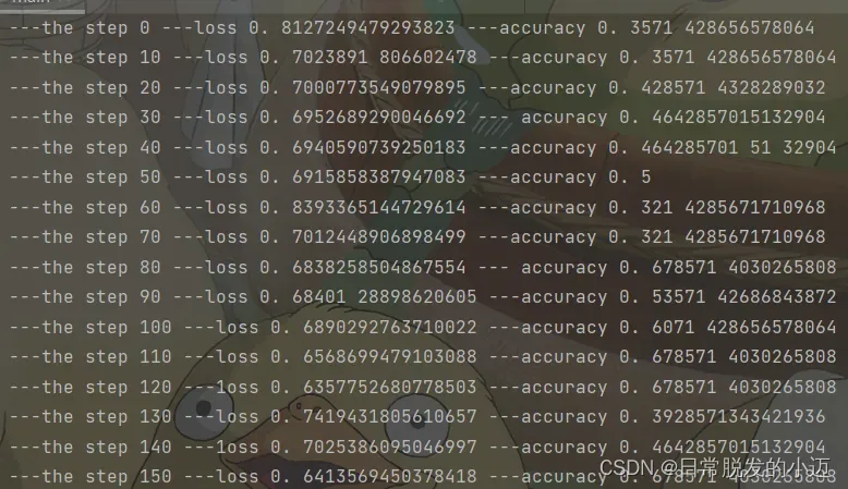
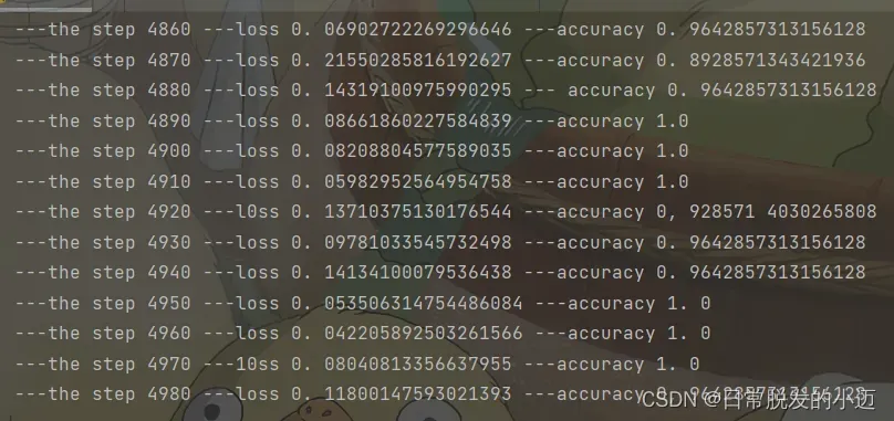
可以看出,当步数(step)为0时,损失率(loss)约为0.8127249479293823,准确率(accuracy)约为0.3571428656578064。随着步数的增加,损失率逐渐下降,趋近于0。准确率逐渐上升,趋近于1。
准确率为通过数据量训练后的label评估来评估模型的预测结果。损失率(loss)为预测之前设计计算后的损失函数的损失值。在模型accuracy里衡量模型的效果为准确分类的样本数与总样本数之比。也就是度量模型的效果。
为了减少优化误差,我们可以计算损失函数,来更新模型参数。所以在优化算法和损失函数的推动下,来减少模型误差风险。比如损失率是我们的课本和考试题知识盲区等内容,让我们去不断消化和学习,来减少我们对知识的盲区,来降低答错率。而准确率就是我们最终的考试成绩。
模型训练结果的可视化结果如下:
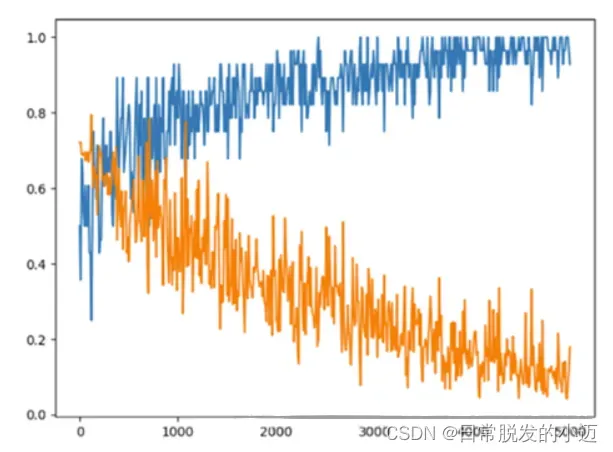
纵轴表示训练的步长,横轴表示概率大小,蓝色表示准确率(accuracy),黄色表示损失率(loss),随着步长的增加,准确率逐渐趋近于1,损失率逐渐趋近于0,模型则越完美。
4.3 识别预测结果
这里利用opencv库,输出图像进行实验验证,代码如下:
#!/usr/bin/env python
# -*- coding: utf-8 -*-

"""
---------------------------------------------------------
    Name:       opencv
    Author:     欧阳紫樱
    Date:       2023-07-02
    Time:       10:49
---------------------------------------------------------
    Software:
                PyCharm
"""

import cv2
import os
import restore
animals = ['cat', 'dog']
l = os.listdir("./test/")
length = len(l)
for i in range(0, length):
    if l[i].endswith(".jpg"):
        image_path = "./test/" + l[i]
        probabilities, animal = restore.Recognize(image_path)
        image = cv2.imread(image_path)
        text = str(animals[animal[0][0]]) + ' --> ' + str(probabilities[0][0])
        cv2.putText(image, text, (10, 50), cv2.FONT_HERSHEY_DUPLEX, 1.0, (255, 255, 255), 1)
        cv2.imshow('', image)
        cv2.waitKey(0)
        cv2.imwrite('./out/' + str(i) + '.jpg', image)
将任意部分测试图像放入test文件夹中,输出结果如下图:
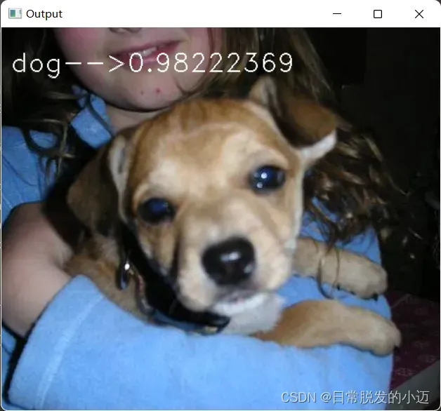
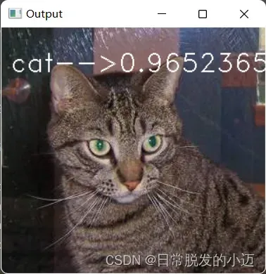
由图可知,在每张图片的头部,显示该图片的特征(猫或狗)和准确率大小(0~1)
准确率大小趋近于1,验证了基于CNN卷积神经网络的图像识别算法的可行性
5 猫狗分类(keras基准模型)
5.1 构建网络模型
与上一节构建模型差不多,这里不做过多讲解,
代码如下:
#网络模型构建
from keras import layers
from keras import models
#keras的序贯模型
model = models.Sequential()
#卷积层,卷积核是3*3,激活函数relu
model.add(layers.Conv2D(32, (3, 3), activation='relu',
                        input_shape=(150, 150, 3)))
#最大池化层
model.add(layers.MaxPooling2D((2, 2)))
#卷积层,卷积核2*2,激活函数relu
model.add(layers.Conv2D(64, (3, 3), activation='relu'))
#最大池化层
model.add(layers.MaxPooling2D((2, 2)))
#卷积层,卷积核是3*3,激活函数relu
model.add(layers.Conv2D(128, (3, 3), activation='relu'))
#最大池化层
model.add(layers.MaxPooling2D((2, 2)))
#卷积层,卷积核是3*3,激活函数relu
model.add(layers.Conv2D(128, (3, 3), activation='relu'))
#最大池化层
model.add(layers.MaxPooling2D((2, 2)))
#flatten层,用于将多维的输入一维化,用于卷积层和全连接层的过渡
model.add(layers.Flatten())
#全连接,激活函数relu
model.add(layers.Dense(512, activation='relu'))
#全连接,激活函数sigmoid
model.add(layers.Dense(1, activation='sigmoid'))
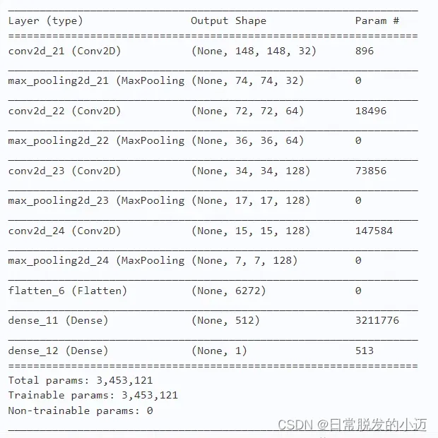
查看模型各层的参数状况:
#输出模型各层的参数状况
model.summary()
Model: "sequential_1"
_________________________________________________________________
Layer (type)                 Output Shape              Param #
=================================================================
conv2d_1 (Conv2D)            (None, 148, 148, 32)      896
_________________________________________________________________
max_pooling2d_1 (MaxPooling2 (None, 74, 74, 32)        0
_________________________________________________________________
conv2d_2 (Conv2D)            (None, 72, 72, 64)        18496
_________________________________________________________________
max_pooling2d_2 (MaxPooling2 (None, 36, 36, 64)        0
_________________________________________________________________
conv2d_3 (Conv2D)            (None, 34, 34, 128)       73856
_________________________________________________________________
max_pooling2d_3 (MaxPooling2 (None, 17, 17, 128)       0
_________________________________________________________________
conv2d_4 (Conv2D)            (None, 15, 15, 128)       147584
_________________________________________________________________
max_pooling2d_4 (MaxPooling2 (None, 7, 7, 128)         0
_________________________________________________________________
flatten_1 (Flatten)          (None, 6272)              0
_________________________________________________________________
dense_1 (Dense)              (None, 512)               3211776
_________________________________________________________________
dense_2 (Dense)              (None, 1)                 513
=================================================================
Total params: 3,453,121
Trainable params: 3,453,121
Non-trainable params: 0
_________________________________________________________________
5.2 训练配置
配置训练方法
from keras import optimizers

model.compile(loss='binary_crossentropy',
              optimizer=optimizers.RMSprop(lr=1e-4),
              metrics=['acc'])
其中,优化器和损失函数可以是字符串形式的名字,也可以是函数形式。
文件中图像转换成所需格式
将训练和验证的图片,调整为150*150
from keras.preprocessing.image import ImageDataGenerator

# 所有图像将按1/255重新缩放
train_datagen = ImageDataGenerator(rescale=1./255)
test_datagen = ImageDataGenerator(rescale=1./255)

train_generator = train_datagen.flow_from_directory(
        # 这是目标目录
        train_dir,
        # 所有图像将调整为150x150
        target_size=(150, 150),
        batch_size=20,
        # 因为我们使用二元交叉熵损失,我们需要二元标签
        class_mode='binary')

validation_generator = test_datagen.flow_from_directory(
        validation_dir,
        target_size=(150, 150),
        batch_size=20,
        class_mode='binary')
Found 2000 images belonging to 2 classes.
Found 1000 images belonging to 2 classes.
查看上述操作处理结果
#查看上面对于图片预处理的处理结果
for data_batch, labels_batch in train_generator:
    print('data batch shape:', data_batch.shape)
    print('labels batch shape:', labels_batch.shape)
    break
data batch shape: (20, 150, 150, 3)
labels batch shape: (20,)
5.3 模型训练
模型训练并保存生成的模型
#模型训练过程
# 模型训练过程
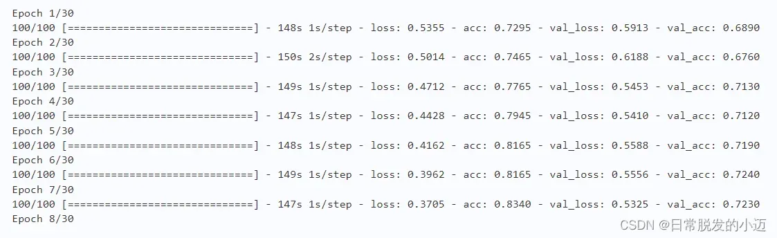
history = model.fit(
train_generator,
steps_per_epoch=100,
epochs=30,
validation_data=validation_generator,
validation_steps=50)
# 保存训练得到的模型
model.save('work/output/cats_and_dogs_small_1.h5')
训练过程如下:
5.4 结果可视化
#对于模型进行评估,查看预测的准确性
import matplotlib.pyplot as plt

acc = history.history['acc']
val_acc = history.history['val_acc']
loss = history.history['loss']
val_loss = history.history['val_loss']

epochs = range(len(acc))

plt.plot(epochs, acc, 'bo', label='Training acc')
plt.plot(epochs, val_acc, 'b', label='Validation acc')
plt.title('Training and validation accuracy')
plt.legend()

plt.figure()

plt.plot(epochs, loss, 'bo', label='Training loss')
plt.plot(epochs, val_loss, 'b', label='Validation loss')
plt.title('Training and validation loss')
plt.legend()

plt.show()
训练时的效果可视化结果如下:
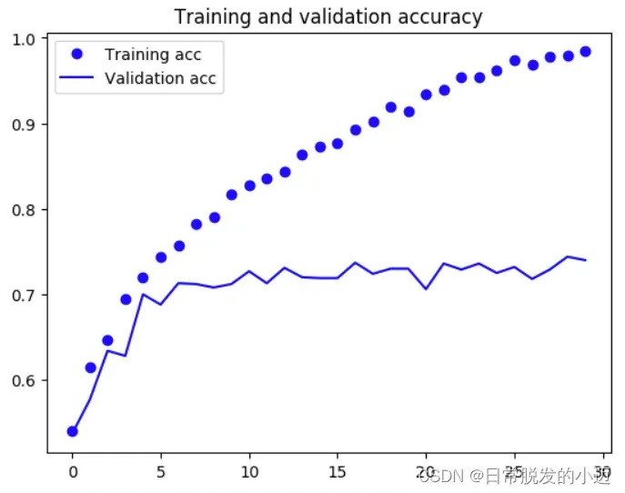
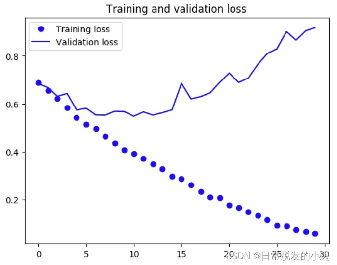
由该效果发现,训练损失值呈上升趋势。即可以得出结论,训练获得的模型存在一些问题,导致了模型过拟合。过拟合是为了得到一致假设而使假设变得过度严格,实际训练得到的模型的分类效果不佳。
6 基准模型的调整
6.1 图像增强
利用图像生成器定义一些常见的图像变换,图像增强就是通过对于图像进行变换,从而,增强图像中的有用信息。
#该部分代码及以后的代码,用于替代基准模型中分类后面的代码(执行代码前,需要先将之前分类的目录删掉,重写生成分类,否则,会发生错误)
from keras.preprocessing.image import ImageDataGenerator
datagen = ImageDataGenerator(
      rotation_range=40,
      width_shift_range=0.2,
      height_shift_range=0.2,
      shear_range=0.2,
      zoom_range=0.2,
      horizontal_flip=True,
      fill_mode='nearest')
①rotation_range
一个角度值(0-180),在这个范围内可以随机旋转图片
②width_shift和height_shift
范围(作为总宽度或高度的一部分),在其中可以随机地垂直或水平地转换图片
③shear_range
用于随机应用剪切转换
④zoom_range
用于在图片内部随机缩放
⑤horizontal_flip
用于水平随机翻转一半的图像——当没有假设水平不对称时(例如真实世界的图片)
⑥fill_mode
用于填充新创建像素的策略,它可以在旋转或宽度/高度移动之后出现
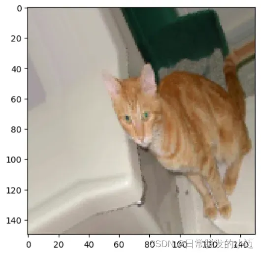
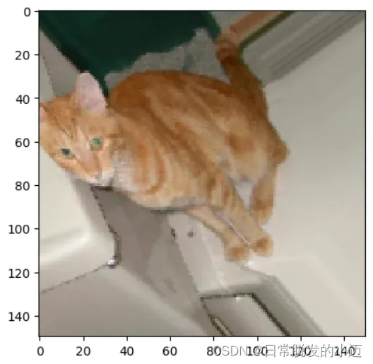
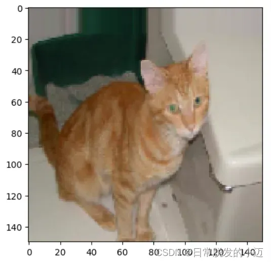
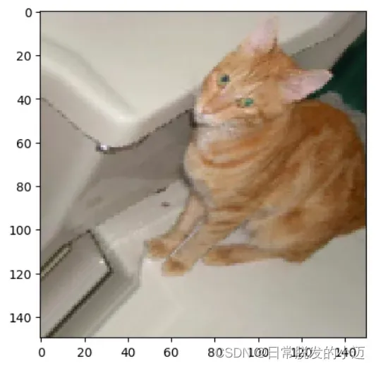
查看增强后的图像
import matplotlib.pyplot as plt
# This is module with image preprocessing utilities
from keras.preprocessing import image
fnames = [os.path.join(train_cats_dir, fname) for fname in os.listdir(train_cats_dir)]
# We pick one image to "augment"
img_path = fnames[3]
# Read the image and resize it
img = image.load_img(img_path, target_size=(150, 150))
# Convert it to a Numpy array with shape (150, 150, 3)
x = image.img_to_array(img)
# Reshape it to (1, 150, 150, 3)
x = x.reshape((1,) + x.shape)
# The .flow() command below generates batches of randomly transformed images.
# It will loop indefinitely, so we need to `break` the loop at some point!
i = 0
for batch in datagen.flow(x, batch_size=1):
    plt.figure(i)
    imgplot = plt.imshow(image.array_to_img(batch[0]))
    i += 1
    if i % 4 == 0:
        break
plt.show()
6.2 添加一层dropout
在网络模型中增加一层dropout
#网络模型构建
from keras import layers
from keras import models
#keras的序贯模型
model = models.Sequential()
#卷积层,卷积核是3*3,激活函数relu
model.add(layers.Conv2D(32, (3, 3), activation='relu',
input_shape=(150, 150, 3)))
#最大池化层
model.add(layers.MaxPooling2D((2, 2)))
#卷积层,卷积核2*2,激活函数relu
model.add(layers.Conv2D(64, (3, 3), activation='relu'))
#最大池化层
model.add(layers.MaxPooling2D((2, 2)))
#卷积层,卷积核是3*3,激活函数relu
model.add(layers.Conv2D(128, (3, 3), activation='relu'))
#最大池化层
model.add(layers.MaxPooling2D((2, 2)))
#卷积层,卷积核是3*3,激活函数relu
model.add(layers.Conv2D(128, (3, 3), activation='relu'))
#最大池化层
model.add(layers.MaxPooling2D((2, 2)))
#flatten层,用于将多维的输入一维化,用于卷积层和全连接层的过渡
model.add(layers.Flatten())
#退出层
model.add(layers.Dropout(0.5))
#全连接,激活函数relu
model.add(layers.Dense(512, activation='relu'))
#全连接,激活函数sigmoid
model.add(layers.Dense(1, activation='sigmoid'))
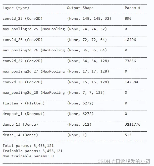
#输出模型各层的参数状况
model.summary()
from keras import optimizers
model.compile(loss='binary_crossentropy',
optimizer=optimizers.RMSprop(lr=1e-4),
metrics=['acc'])
下图为不添加dropout和添加dropout的结构对比:
6.3 训练模型
train_datagen = ImageDataGenerator(
    rescale=1./255,
    rotation_range=40,
    width_shift_range=0.2,
    height_shift_range=0.2,
    shear_range=0.2,
    zoom_range=0.2,
    horizontal_flip=True,)
# Note that the validation data should not be augmented!
test_datagen = ImageDataGenerator(rescale=1./255)
train_generator = train_datagen.flow_from_directory(
        # This is the target directory
        train_dir,
        # All images will be resized to 150x150
        target_size=(150, 150),
        batch_size=32,
        # Since we use binary_crossentropy loss, we need binary labels
        class_mode='binary')
validation_generator = test_datagen.flow_from_directory(
        validation_dir,
        target_size=(150, 150),
        batch_size=32,
        class_mode='binary')
history = model.fit_generator(
      train_generator,
      steps_per_epoch=100,
      epochs=100,
      validation_data=validation_generator,
      validation_steps=50)
model.save('G:\\Cat_And_Dog\\kaggle\\cats_and_dogs_small_2.h5')
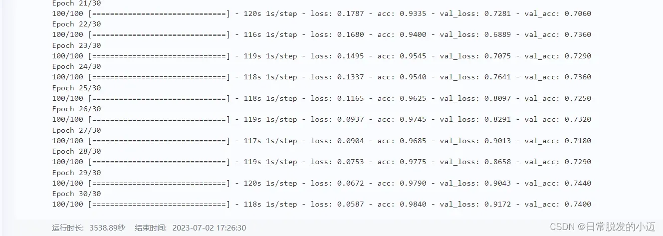
训练过程如下:
结果可视化:
acc = history.history['acc']
val_acc = history.history['val_acc']
loss = history.history['loss']
val_loss = history.history['val_loss']
epochs = range(len(acc))
plt.plot(epochs, acc, 'bo', label='Training acc')
plt.plot(epochs, val_acc, 'b', label='Validation acc')
plt.title('Training and validation accuracy')
plt.legend()
plt.figure()
plt.plot(epochs, loss, 'bo', label='Training loss')
plt.plot(epochs, val_loss, 'b', label='Validation loss')
plt.title('Training and validation loss')
plt.legend()
plt.show()
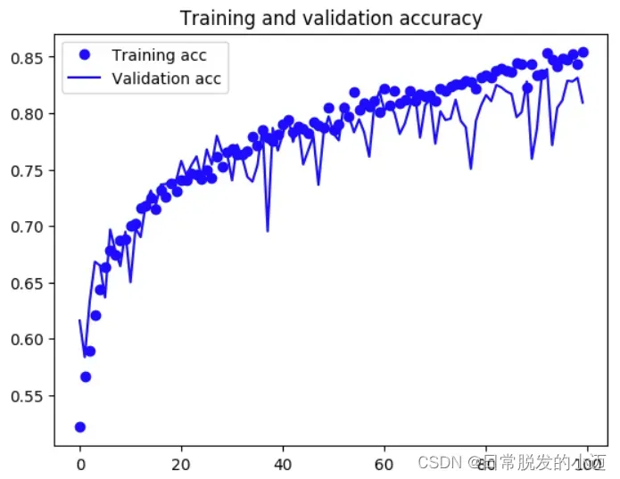
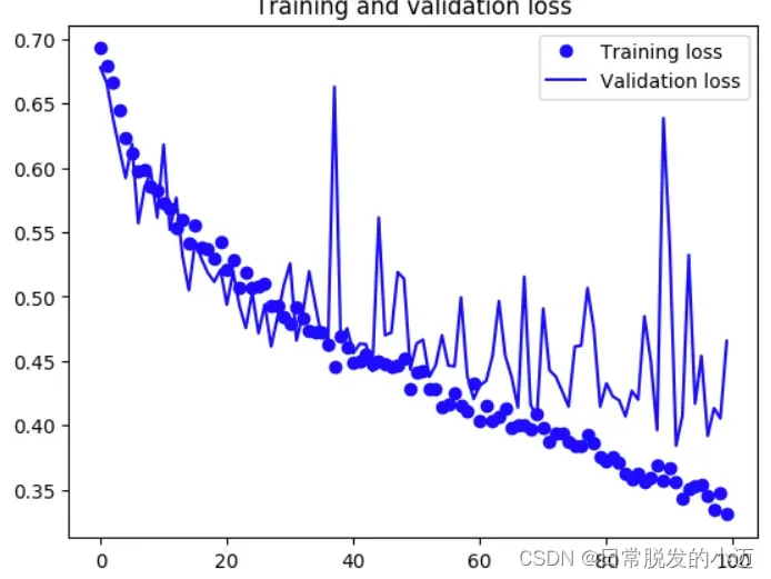
根据上图可知,对比基准模型,可以很清楚的发现loss的整体趋势是变小的。只进行图像增强获得的模型和进行图像增强与添加dropout层获得的模型,可以发现前者在训练过程中波动会更大,后者在准确上小于前者。两者虽然在准确率有所变小,但是都避免了过拟合。
总结
通过本次实验,我们深入了解了CNN模型的应用,并通过数据增强和dropout层等技术提升了模型的性能和鲁棒性。通过实验我们发现,仅仅进行数据增强操作可以显著提高模型的精确率。数据增强能够有效地增加训练样本的数量,并使模型更好地学习数据的特征,从而提高分类准确性。
参考:
https://blog.csdn.net/weixin_44404350/article/details/116292586
https://blog.csdn.net/kevinjin2011/article/details/124944728
https://blog.csdn.net/qq_43279579/article/details/117298169
文章出处登录后可见!