【论文精读】Benchmarking Deep Learning Interpretability in Time Series Predictions

Abstract

Saliency methods are used extensively to highlight the importance of input features in model predictions. These methods are mostly used in vision and language tasks, and their applications to time series data is relatively unexplored. In this paper, we set out to extensively compare the performance of various saliency-based interpretability methods across diverse neural architectures, including Recurrent Neural Network, Temporal Convolutional Networks, and Transformers in a new benchmark of synthetic time series data. We propose and report multiple metrics to empirically evaluate the performance of saliency methods for detecting feature importance over time using both precision (i.e., whether identified features contain meaningful signals) and recall (i.e., the number of features with signal identified as important). Through several experiments, we show that
(i) in general, network architectures and saliency methods fail to reliably and accurately identify feature importance over time in time series data,
(ii) this failure is mainly due to the conflation of time and feature domains, and
(iii) the quality of saliency maps can be improved substantially by using our proposed two-step temporal saliency rescaling (TSR) approach that first calculates the importance of each time step before calculating the importance of each feature at a time step.

显著性方法Saliency methods被广泛用于强调模型预测中输入特征的重要性。这些方法主要用于视觉和语言任务，它们在时间序列数据上的应用还相对未被探索。在本文中，我们着手在不同的神经架构上广泛比较各种基于显著性的可解释性方法的性能，包括循环神经网络Recurrent Neural Network、时态卷积网络Temporal Convolutional Networks和Transformers在合成时间序列数据的新基准中。
我们提出并报告了多个指标，以经验地评估显著性方法的性能，使用精度precision(即，识别的特征是否包含有意义的信号)和召回率recall(即，信号被识别为重要的特征的数量)来检测特征的重要性。通过多次实验，我们证明:
(i)总体而言，网络架构和显著性方法无法可靠准确地识别时间序列数据中特征重要性随时间的变化，
(ii)这种失败主要是由于时间和特征域的合并，
(iii)显著性图saliency maps的质量可以通过使用我们提出的两步时间显著性重新缩放(two-step temporal saliency
rescaling TSR)方法大幅提高，该方法首先计算每个时间步的重要性，然后计算每个时间步的每个特征的重要性。

1 Introduction

As the use of Machine Learning models increases in various domains [1, 2], the need for reliable model explanations is crucial [3, 4]. This need has resulted in the development of numerous interpretability methods that estimate feature importance [5–13]. As opposed to the task of understanding the prediction performance of a model, measuring and understanding the performance of interpretability methods is challenging [14–18] since there is no ground truth to use for such comparisons. For instance, while one could identify sets of informative features for a specific task a priori, models may not necessarily have to draw information from these features to make accurate predictions. In multivariate time series data, these challenges are even more profound since we cannot rely on human perception as one would when visualizing interpretations by overlaying saliency maps over images or when highlighting relevant words in a sentence.

随着机器学习模型在各个领域的使用的增加[1,2]，对可靠模型解释的需求是至关重要的[3,4]。这种需求导致了许多估计特征重要性的可解释性方法的发展[5-13]。与理解模型的预测性能相反，测量和理解可解释性方法的性能具有挑战性[14-18]，因为没有用于此类比较的标准答案ground truth。
例如，虽然人们可以先验地为特定任务识别一组信息特征，但模型可能不一定要从这些特征中提取信息来做出准确的预测。在多元时间序列数据中，这些挑战甚至更加深刻，因为我们不能像在图像上叠加显著性图或在句子中突出相关单词时那样依赖于人类的感知。

In this work, we compare the performance of different interpretability methods both perturbation-based and gradient-based methods, across diverse neural architectures including Recurrent Neural Network, Temporal Convolutional Networks, and Transformers when applied to the classification of multivariate time series. We quantify the performance of every (architectures, estimator) pair for time series data in a systematic way. We design and generate multiple synthetic datasets to capture different temporal-spatial aspects (e.g., Figure 1). Saliency methods must be able to distinguish important and non-important features at a given time, and capture changes in the importance of features over time. The positions of informative features in our synthetic datasets are known a priori (colored boxes in Figure 1); however, the model might not need all informative features to make a prediction. To identify features needed by the model, we progressively mask the features identified as important by each interpretability method and measure the accuracy degradation of the trained model.
We then calculate the precision and recall for (architectures, estimator) pairs at different masks by comparing them to the known set of informative features.

在这项工作中，我们比较了不同的可解释性方法，包括基于扰动的方法perturbation-based和基于梯度的方法gradient-based，在不同的神经架构中，包括循环神经网络Recurrent Neural Network、时态卷积网络Temporal Convolutional Networks和Transformers，当应用于多元时间序列multivariate time series分类时的性能。我们以系统的方式量化时间序列数据的每个(架构，估计器)对的性能。我们设计并生成多个合成数据集来捕捉不同的时间-空间方面(例如，图1)。

显著性方法 Saliency methods必须能够在给定时间区分重要和不重要的特征，并捕捉特征重要性随时间的变化。信息特征在我们的合成数据集中的位置是先验已知的(图1中的彩色方框);然而，该模型可能不需要所有的信息特征来进行预测。

为了识别模型所需的特征，我们逐步屏蔽由每种可解释性方法识别为重要的特征，并测量训练模型的精度退化。然后，通过将(架构，估计器)对与已知的信息特征集进行比较，计算不同掩码下(架构，估计器)对的精度和召回率。

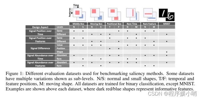
Figure 1: Different evaluation datasets used for benchmarking saliency methods. Some datasets have multiple variations shown as sub-levels. N/S: normal and small shapes, T/F: temporal and feature positions, M: moving shape. All datasets are trained for binary classification, except MNIST.
Examples are shown above each dataset, where dark red/blue shapes represent informative features.
图1:用于基准显著性方法的不同评估数据集。一些数据集有多个变量，显示为子级别。N/S:正常形状和小形状，T/F:时间和特征位置，M:移动形状。除MNIST外，所有数据集都进行了二进制分类训练。每个数据集上面显示了示例，其中深红/蓝色形状表示信息特征。

Based on our extensive experiments, we report the following observations:
(i) feature importance estimators that produce high-quality saliency maps in images often fail to provide similar high-quality interpretation in time series data,
(ii) saliency methods tend to fail to distinguish important vs. nonimportant features in a given time step; if a feature in a given time is assigned to high saliency, then almost all other features in that time step tend to have high saliency regardless of their actual values,
(iii) model architectures have significant effects on the quality of saliency maps.

基于我们广泛的实验，我们报告了以下观察结果:
(i)在图像中产生高质量显著性图的特征重要性估计器通常无法在时间序列数据中提供类似的高质量解释，
(ii)显著性方法往往无法在给定的时间步长中区分重要与不重要的特征;如果给定时间内的一个特征被分配为高显著性，那么该时间步中的几乎所有其他特征都倾向于具有高显著性，而不管它们的实际值如何，
(iii)模型架构对显著性图的质量有显著影响。

After the aforementioned analysis and to improve the quality of saliency methods in time series data, we propose a two-step Temporal Saliency Rescaling (TSR) approach that can be used on top of any existing saliency method adapting it to time series data. Briefly, the approach works as follows:
(a) we first calculate the time-relevance score for each time by computing the total change in saliency values if that time step is masked; then
(b) in each time-step whose time-relevance score is above a certain threshold, we calculate the feature-relevance score for each feature by computing the total change in saliency values if that feature is masked. The final (time, feature) importance score is the product of associated time and feature relevance scores. This approach substantially improves the quality of saliency maps produced by various methods when applied to time series data. Figure 4 shows the initial performance of multiple methods, while Figure 5 shows their performance coupled with our proposed TSR method.

在上述分析之后，为了提高时间序列数据中显著性方法的质量，我们提出了一种两步时态显著性重新缩放(TSR) two-step Temporal Saliency Rescaling方法，可以在任何现有的显著性方法之上使用，使其适应时间序列数据。简单地说，该方法的工作原理如下:
(a)我们首先通过计算显着性值的总变化来计算每个时间的时间相关性得分，
如果该时间步长被掩盖;然后
(b)在每个时间步中，如果时间相关性得分高于某个阈值，我们通过计算显著性值的总变化来计算每个特征的特征相关性得分，如果该特征被掩盖。
最终的(时间，特征)重要性得分是相关时间和特征相关性得分的乘积。当应用于时间序列数据时，这种方法极大地提高了由各种方法生成的显著性图的质量。
图4显示了多种方法的初始性能，
而图5显示了它们与我们提出的TSR方法相结合的性能。

2 Background and Related Work

The interest in interpretability resulted in several diverse lines of research, all with a common goal of understanding how a network makes a prediction. [19–23] focus on making neural models more interpretable. [24, 9, 11, 6, 7, 25] estimate the importance of an input feature for a specified output.
Kim et al [26] provides an interpretation in terms of human concepts. One key question is whether or not interpretability methods are reliable. Kindermans et al [17] shows that the explanation can be manipulated by transformations that do not affect the decision-making process. Ghorbani et al
[15] introduces an adversarial attack that changes the interpretation without changing the prediction.
Adebayo et al [16] measures changes in the attribute when randomizing model parameters or labels.
Similar to our line of work, modification-based evaluation methods [27–29] involves: applying saliency method, ranking features according to the saliency values, recursively eliminating higher ranked features and measure degradation to the trained model accuracy. Hooker et al [14] proposes retraining the model after feature elimination.
Recent work [23, 30, 31] have identified some limitations in time series interpretability. We provide the first benchmark that systematically evaluates different saliency methods across multiple neural architectures in a multivariate time series setting, identifies common limitations, and proposes a solution to adapt existing methods to time series.

对可解释性的兴趣导致了几种不同的研究方向，所有这些研究都有一个共同的目标，即理解网络如何进行预测。

[19-23]致力于使神经模型更具可解释性。[24,9,11,6,7,25]估计输入特征对指定输出的重要性。
Kim et al[26]从人类概念的角度进行了解释。一个关键问题是可解释性方法是否可靠。
Kindermans等[17]表明，解释可以被不影响决策过程的转换所操纵。
Ghorbani等人[15]引入了一种对抗性攻击，在不改变预测的情况下改变解释。
Adebayo et al[16]在随机化模型参数或标签时测量属性的变化。

与我们的工作类似，基于修改的评估方法[27-29]包括:应用显著性方法，根据显著性值对特征进行排名，递归地消除排名较高的特征，并测量训练模型精度的退化。
Hooker等[14]提出在特征消除后对模型进行再训练。
最近的研究[23,30,31]指出了时间序列可解释性的一些局限性。
我们提供了第一个基准，系统地评估了多元时间序列设置中跨多个神经架构的不同显著性方法，确定了常见的局限性，并提出了一种解决方案，使现有方法适应时间序列。

2.1 Saliency Methods

We compare popular backpropagation-based and perturbation based post-hoc saliency methods; each method provides feature importance, or relevance, at a given time step to each input feature. All methods are compared with random assignment as a baseline control.
In this benchmark, the following saliency methods† are included:

• Gradient-based: Gradient (GRAD) [5] the gradient of the output with respect to the input. Integrated Gradients (IG) [9] the average gradient while input changes from a non-informative reference point. SmoothGrad (SG) [10] the gradient is computed n times, adding noise to the input each time. DeepLIFT (DL) [11] defines a reference point, relevance is the difference between the activation of each neuron to its reference activation. Gradient SHAP (GS) [12] adds noise to each input, selects a point along the path between a reference point and input, and computes the gradient of outputs with respect to those points. Deep SHAP (DeepLIFT + Shapley values) (DLS) [12] takes a distribution of baselines computes the attribution for each input-baseline pair and averages the resulting attributions per input.

• Perturbation-based: F eature Occlusion (FO) [24] computes attribution as the difference in output after replacing each contiguous region with a given baseline. For time series we considered continuous regions as features with in same time step or multiple time steps grouped together. F eature Ablation (F A) [32] computes attribution as the difference in output after replacing each feature with a baseline. Input features can also be grouped and ablated together rather than individually. F eature permutation (FP) [33] randomly permutes the feature value individually, within a batch and computes the change in output as a result of this modification.

• Other: Shapley V alue Sampling (SVS) [34] an approximation of Shapley values that involves sampling some random permutations of the input features and average the marginal contribution of features based the differences on these permutations.

我们比较了流行的
基于反向传播backpropagation-based和
基于扰动perturbation based的
事后post-hoc显著性方法;
每种方法在给定的时间步骤中为每个输入特征提供特征的重要性或相关性。
所有方法均以随机分配作为基线对照。

在这个基准测试中，包括以下显着性方法:

• Gradient-based基于梯度:
  Gradient(GRAD)[5]输出相对于输入的梯度。综合梯度Integrated Gradients(IG)[9]当输入从非信息参考点变化时的平均梯度。
  SmoothGrad (SG)[10]梯度计算n次，每次都向输入添加噪声。
  DeepLIFT (DL)[11]定义了一个参考点，相关性是每个神经元的激活与其参考激活之间的差异。
  Gradient SHAP (GS)[12]为每个输入添加噪声，沿着参考点和输入之间的路径选择一个点，并计算输出相对于这些点的梯度。
  Deep SHAP (DeepLIFT + Shapley值)(DLS)[12]采用基线分布计算每个输入-基线对的属性，并对每个输入的结果属性求平均。

• Perturbation-based基于扰动:
  Feature Occlusion(FO)[24]计算属性作为用给定基线替换每个连续区域后的输出差异。对于时间序列，我们将连续区域视为同一时间步长或多个时间步长组合在一起的特征。
  Feature Ablation(FA)[32]计算属性为用基线替换每个特征后输出的差异。输入特征也可以分组并一起消融，而不是单独。
  Feature permutation (FP)[33]在批处理中随机地逐个排列特征值，并计算这种修改导致的输出变化。

• 其他:Shapley值采样Shapley Value Sampling(SVS)[34]沙普利值的近似值，包括对输入特征的一些随机排列进行采样，并根据这些排列的差异平均特征的边际贡献。

2.2 Neural Net Architectures

In this benchmark, we consider 3 main neural architectures groups; Recurrent networks, Convolution neural networks (CNN) and Transformer. For each group we investigate a subset of models that are commonly used for time series data. Recurrent models include: LSTM [35] and LSTM with Input-Cell Attention [23] a variant of LSTM with that attends to inputs from different time steps.
For CNN, Temporal Convolutional Network (TCN) [36–38] a CNN that handles long sequence time series. Finally, we consider the original Transformers [39] implementation.

在这个基准测试中，我们考虑了3个主要的神经架构组;
循环网络(RNN)，卷积神经网络(CNN)和Transformers。
对于每一组，我们研究了通常用于时间序列数据的模型子集。

循环模型包括:LSTM[35]和LSTM with Input-Cell Attention [23]， LSTM的一种变体，用于处理来自不同时间步的输入。

对于CNN，时态卷积网络(Temporal Convolutional Network, TCN)[36-38]是一种处理长序列时间序列的CNN。

最后，我们考虑原始的Transformers[39]实现。

Problem Definition

We study a time series classification problem where all time steps contribute to making the final output; labels are available after the last time step. In this setting, a network takes multivariate time series input X = [x1, . . . , xT ] ∈ RN×T , where T is the number of time steps and N is the number of features. Let xi,t be the input feature i at time t. Similarly, let X:,t ∈ RN and Xi,: ∈ RT be the feature vector at time t, and the time vector for feature i, respectively. The network produces an output S(X) = [S1(X), …, SC(X)], where C is the total number of classes (i.e. outputs). Given a target class c, the saliency method finds the relevance R(X) ∈ RN×T which assigns relevance scores Ri,t(X) for input feature i at time t.

我们研究了一个时间序列分类问题，其中所有的时间步长都有助于产生最终的输出;标签在最后一个时间步骤之后可用。在此设置中，网络接受多元时间序列输入，其中T为时间步数，N为特征数。设xi,t为t时刻的输入特征i。同理，设X:，t∈RN, xi，:∈RT为t时刻的特征向量，xi，:∈RT为特征i的时间向量。网络产生输出S(X) = [S1(X)，…， SC(X)]，其中C是类的总数(即输出)。给定一个目标类c，显著性方法找到相关性R(X)∈RN×T，它为t时刻的输入特征i分配相关性分数Ri,t(X)。

4 Benchmark Design and Evaluation Metrics

4.1 Dataset Design

Since evaluating interpretability through saliency maps in multivariate time series datasets is nontrivial, we design multiple synthetic datasets where we can control and examine different design aspects that emerge in typical time series datasets. We extend the synthetic data proposed by Ismail et al [23] for binary classification. We consider how the discriminating signal is distributed over both time and feature axes, reflecting the importance of time and feature dimensions separately. We also examine how the signal is distributed between classes: difference in value, position, or shape. Additionally, we modify the classification difficulty by decreasing the number of informative features (reducing feature redundancy), i.e., small box datasets. Along with synthetic datasets, we included MNIST as a multivariate time series as a more general case (treating one of the image axes as time). Different dataset combinations are shown in Figure 1.

由于在多元时间序列数据集中通过显著性图评估可解释性并非易事，因此我们设计了多个合成数据集，在这些数据集中，我们可以控制和检查典型时间序列数据集中出现的不同设计方面。
我们扩展了Ismail等[23]提出的合成数据用于二元分类。我们考虑了区分信号如何在时间轴和特征轴上分布，分别反映了时间和特征维度的重要性。
我们还研究了信号在类之间是如何分布的:值、位置或形状的差异。此外，我们通过减少信息特征的数量(减少特征冗余)来修改分类难度，即小盒数据集。除了合成数据集，我们还将MNIST作为多元时间序列作为更一般的情况(将图像轴中的一个作为时间)。不同的数据集组合如图1所示。

Each synthetic dataset is generated by seven different processes as shown in Figure 2, giving a total of 70 datasets. Each feature is independently sampled from either:
(a) Gaussian with zero mean and unit variance.
(b) Independent sequences of a standard autoregressive time series with Gaussian noise.
( c ) A standard continuous autoregressive time series with Gaussian noise.
(d) Sampled according to a Gaussian Process mixture model.
(e) Nonuniformly sampled from a harmonic function.
(f) Sequences of standard non–linear autoregressive moving average (NARMA) time series with Gaussian noise.
(g) Nonuniformly sampled from a pseudo period function with Gaussian noise. Informative features are then highlighted by the addition of a constant µ to positive class and subtraction of µ from negative class (unless specified, µ = 1); the embedding size for each sample is N = 50, and the number of time steps is T = 50. Figures throughout the paper show data generated as Gaussian noise unless otherwise specified. Further details are provided in the supplementary material.

每个合成数据集由7个不同的过程生成，如图2所示，总共有70个数据集。每个特征都是独立采样的:
(a)均值为零，单位方差为零的高斯分布。
(b)带有高斯噪声的标准自回归时间序列的独立序列。
(c )具有高斯噪声的标准连续自回归时间序列。
(d)根据高斯过程混合模型采样。
(e)从谐波函数中非均匀采样。
(f)带有高斯噪声的标准非线性自回归移动平均时间序列序列。
(g)从具有高斯噪声的伪周期函数中非均匀采样。然后，通过在正类中添加常数µ和从负类中减去µ(除非指定，µ= 1)来突出信息特征;每个样本的嵌入大小为N = 50，时间步数为T = 50。除非另有说明，本文中的图都是作为高斯噪声生成的数据。进一步的细节载于补充材料。

4.2 Feature Importance Identification

Modification-based evaluation metrics [27–29] have two main issues. First, they assume that feature ranking based on saliency faithfully represents feature importance. Consider the saliency distributions shown in Figure 3. Saliency decays exponentially with feature ranking, meaning that features that are closely ranked might have substantially different saliency values. A second issue, as discussed by Hooker et al [14], is that eliminating features changes the test data distribution violating the assumption that both training and testing data are independent and identically distributed (i.i.d.).
Hence, model accuracy degradation may be a result of changing data distribution rather than removing salient features. In our synthetic dataset benchmark, we address these two issues by the following:

• Sort relevance , so that is the element in ordered set .
• Find top relevant features in the order set such that (where is a pre-determined percentage).
• Replace , where with the original distribution (known since this is a synthetic dataset).
• Calculate the drop in model accuracy after the masking, this is repeated at different values of .

基于修改的评价指标[27-29]有两个主要问题。
首先，他们假设基于显著性的特征排名忠实地代表了特征的重要性。考虑图3所示的显著性分布。显著性随特征排名呈指数级衰减，这意味着排名紧密的特征可能具有本质上不同的显著性值。
第二个问题，正如Hooker等[14]所讨论的，消除特征改变了测试数据的分布，违反了训练数据和测试数据都是独立和同分布(i.i.d)的假设。

因此，模型精度下降可能是改变数据分布的结果，而不是去除显著特征的结果。在我们的合成数据集基准测试中，我们通过以下方式解决这两个问题:

• 排序相关性，使 is the 是有序集 中的第个元素。
• 找到顺序集中的前个相关特征，使得 (其中是预先确定的百分比)。
• 替换，其中 与原始分布(已知，因为这是一个合成数据集)。
• 计算掩蔽后模型精度的下降，这是重复的不同值 。

We address the first issue by removing features that represent a certain percentage of the overall saliency rather than removing a constant number of features. Since we are using synthetic data and masking using the original data distribution, we are not violating i.i.d. assumptions.

我们通过删除代表整体显著性一定百分比的特征来解决第一个问题，而不是删除恒定数量的特征。由于我们使用合成数据并使用原始数据分布进行屏蔽，因此我们没有违反i.i.d.假设。

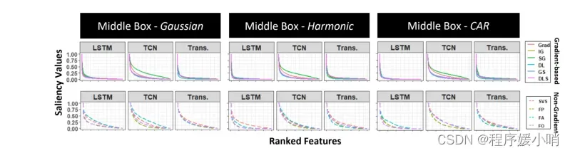
Figure 3: The saliency distribution of ranked features produced by different saliency methods for three variations of the Middle Box dataset (Gaussian, Harmonic, Continous Autoregressive (CAR)).Top row shows gradient-based saliency methods while bottom row shows the rest.

图3:对于中间盒子数据集的三种变化(高斯、谐波、连续自回归(CAR))，由不同显著性方法产生的排名特征的显著性分布。上面一行显示了基于梯度的显著性方法，而下面一行显示了其余的方法。

4.3 Performance Evaluation Metrics

Masking salient features can result in
(a) a steep drop in accuracy, meaning that the removed feature is necessary for a correct prediction or
(b) unchanged accuracy. The latter may result from the saliency method incorrectly identifying the feature as important, or that the removal of that feature is not sufficient for the model to behave incorrectly. Some neural architectures tend to use more feature information when making a prediction (i.e., have more recall in terms of importance); this may be the desired behavior in many time series applications where importance changes over time, and the goal of using an interpretability measure is to detect all relevant features across time.
On the other hand, in some situations, where sparse explanations are preferred, then this behavior may not be appropriate.

掩盖显著特征会导致
(a)精度的急剧下降，这意味着被移除的特征对于正确的预测是必要的;或
(b)精度不变。
后者可能是由于显著性方法错误地将特征识别为重要的，或者删除该特征不足以使模型行为不正确。一些神经结构在进行预测时倾向于使用更多的特征信息(即，在重要性方面有更多的回忆);这可能是许多时间序列应用程序所期望的行为，这些应用程序的重要性随着时间的推移而变化，使用可解释性度量的目标是检测所有相关的特征。
另一方面，在某些情况下，sparse explanations是首选，那么这种行为可能是不合适的。

This in mind, one should not compare saliency methods solely on the loss of accuracy after masking.
Instead, we should look into features identified as salient and answer the following questions:
(1) Are all features identified as salient informative? (precision)
(2) Was the saliency method able to identify all informative features? (recall)
We choice to report the weighted precision and recall of each (neural architecture, saliency method) pair, since, the saliency value varies dramatically across features Figure 3 (detailed calculations are available in the supplementary material).
Through our experiments, we report area under the precision curve (AUP), the area under the recall curve (AUR), and area under precision and recall (AUPR). The curves are calculated by the precision/recall values at different levels of degradation. We also consider feature/time precision and recall (a feature is considered informative if it has information at any time step and vice versa). For the random baseline, we stochastically select a saliency method then permute the saliency values producing arbitrary ranking.

记住这一点，人们不应该只比较显着性方法在掩蔽后的准确性损失。

相反，我们应该研究被认为是突出的特征，并回答以下问题:
(1)所有被认为是突出的特征都有信息吗?(精度)
(2)显著性方法是否能够识别所有的信息特征?(召回率)

我们选择报告每个(神经结构，显著性方法)对的加权精度和召回率，因为，显著性值在特征之间变化很大(详细计算可在补充材料中获得)。

通过我们的实验，我们报告了精度曲线下面积(AUP)，召回曲线下面积(AUR)，以及精度和召回面积(AUPR)。曲线计算精度/召回值在不同程度的退化。我们还考虑了特征/时间精度和召回率(如果一个特征在任何时间步骤都有信息，那么它就被认为是有信息的，反之亦然)。对于随机基线，我们随机选择一种显著性方法，然后对显著性值进行排列，产生任意排序。

5 Saliency Methods Fail in Time Series Data

Due to space limitations, only a subset of the results is reported below; the full set is available in the supplementary material. The results reported in the following section are for models that produce accuracy above 95% in the classification task.

由于篇幅所限，下面只报告部分结果;全套在补充资料中。下一节中报告的结果适用于在分类任务中产生95%以上准确率的模型。

5.1 Saliency Map Quality

Consider synthetic examples in Figure 4; given that the model was able to classify all the samples correctly, one would expect a saliency method to highlight only informative features. However, we find that for the Middle Box and Rare Feature datasets, many different (neural architecture, saliency method) pairs are unable to identify informative features. For Rare time, methods identify the correct time steps but are unable to distinguish informative features within those times. Similarly, methods were not able to provide quality saliency maps produced for the multivariate time series MNIST digit.
Overall most (neural architecture, saliency method) pairs fail to identify importance over time.

考虑图4中的综合例子;鉴于该模型能够正确地对所有样本进行分类，人们会期望显著性方法只突出信息特征。然而，我们发现对于中间框和罕见特征数据集，许多不同的(神经结构，显著性方法)对无法识别信息特征。对于稀有时间，方法识别正确的时间步长，但无法在这些时间内区分信息特征。同样，方法无法提供为多元时间序列MNIST数字生成的高质量显著性图。

总的来说，大多数(神经结构，显著性方法)配对都不能随着时间的推移识别重要性。

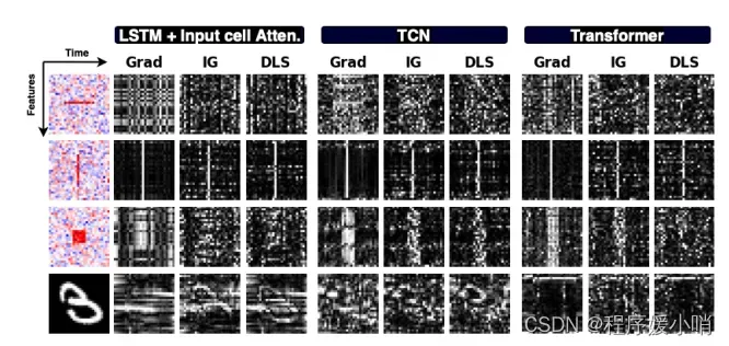
Figure 4: Saliency maps produced by Grad, Integrated Gradients, and DeepSHAP for 3 different models on synthetic data and time series MNIST (white represents high saliency). Saliency seems to highlight the correct time step in some cases but fails to identify informative features in a given time.

图4:Grad、Integrated Gradients和DeepSHAP为合成数据和时间序列MNIST的3个不同模型制作的显著性图(白色表示高显著性)。在某些情况下，显着性似乎突出了正确的时间步长，但无法识别给定时间内的信息特征。

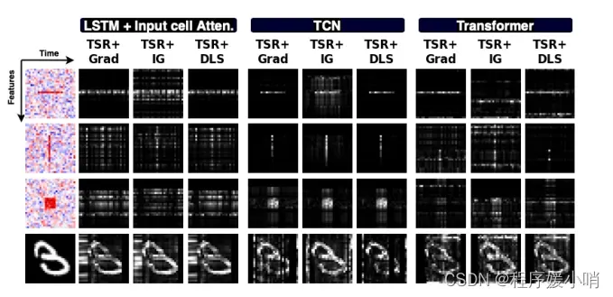
Figure 5: Saliency maps when applying the proposed Temporal Saliency Rescaling (TSR) approach.

图5:应用提议的时态显著性重新缩放(TSR)方法时的显著性图。

5.2 Saliency Methods versus Random Ranking

Here we look into distinctions between each saliency method and a random ranking baseline. The effect of masking salient features on the model accuracy is shown in Figure 6. In a given panel, the leftmost curve indicates the saliency method that highlights a small number of features that impact accuracy severely (if correct, this method should have high precision); the rightmost curve indicates the saliency method that highlights a large number of features that impact accuracy severely (if correct, this method should show high recall).

在这里，我们看看每种显著性方法和随机排名基线之间的区别。掩蔽显著特征对模型精度的影响如图6所示。在给定的面板中，最左边的曲线表示显著性方法，该方法突出少量严重影响精度的特征(如果正确，该方法应该具有较高的精度);最右边的曲线表示显著性方法，突出大量严重影响准确性的特征(如果正确，这种方法应该显示高召回率)。

Model Accuracy Drop

We were unable to identify a consistent trend for saliency methods across all neural architectures throughout experiments. Instead, saliency methods for a given architecture behave similarly across datasets. E.g., in TCN Grad and SmoothGrad had steepest accuracy drop across all datasets while LSTM showed no clear distinction between random assignment and non-random saliency method curves (this means that LSTM is very hard to interpret regardless of the saliency method used as [23]) V ariance in performance between methods can be explained by the dataset itself rather than the methods. E.g., the Moving box dataset showed minimal variance across all methods, while Rare time dataset showed the highest.

在整个实验过程中，我们无法在所有神经结构中确定显著性方法的一致趋势。相反，给定体系结构的显著性方法在数据集之间的行为类似。
例如，在TCN中，Grad和SmoothGrad在所有数据集上的精度下降幅度最大，而LSTM在随机分配和非随机显著性方法曲线之间没有明显的区别(这意味着LSTM很难解释，不管[23]使用的是显著性方法)，方法之间的性能差异可以用数据集本身而不是方法来解释。例如，Moving box数据集在所有方法中表现出最小的方差，而Rare time数据集表现出最高的方差。

Precision and Recall

Looking at precision and recall distribution box plots Figure 7 (the precision and recall graphs per dataset are available in the supplementary materials), we observe the following:
(a) Model architecture has the largest effect on precision and recall.
(b) Results do not show clear distinctions between saliency methods.
(c ) Methods can identify informative time steps while fail to identify informative features; AUPR in the time domain (second-row Figure 7) is higher than that in the feature domain (third-row Figure 7).
(d) Methods identify most features in an informative time step as salient, AUR in feature domain is very high while having very low AUP . This is consistent with what we see in Figure 4, where all features in informative time steps are highlighted regardless of there actual values.
(e) Looking at AUP , AUR, and AUPR values, we find that the steepness in accuracy drop depends on the dataset. A steep drop in model accuracy does not indicate that a saliency method is correctly identifying features used by the model since, in most cases, saliency methods with leftmost curves in Figure 6 have the lowest precision and recall values.

查看精度和召回率分布盒图图7(每个数据集的精度和召回率图可在补充材料中获得)，我们观察到以下几点:
(a)模型架构对精度和召回率的影响最大。
(b)显著性方法的结果差异不明显。
(c )方法可以识别信息性时间步长，但不能识别信息性特征;时域的AUPR(图7第二行)高于特征域的AUPR(图7第三行)。
(d)方法识别信息时间步中的大多数特征为显著性，特征域的AUR非常高，但AUP非常低。这与我们在图4中看到的一致，在图4中，无论实际值如何，信息时间步骤中的所有功能都被突出显示。
(e)查看AUP、AUR和AUPR值，我们发现精度下降的陡度取决于数据集。模型精度的急剧下降并不表明显著性方法正确地识别了模型所使用的特征，因为在大多数情况下，图6中最左侧曲线的显著性方法具有最低的精度和召回值。

6 Saliency Maps for Images versus Multivariate Time Series

Since saliency methods are commonly evaluated on images, we compare the saliency maps produced from models like CNN, which fit images, to the maps produced by temporal models like TCN, over our evaluation datasets by treating the complete multivariate time series as an image. Figure 8(a) shows two examples of such saliency maps. The maps produced by CNN can distinguish informative pixels corresponding to informative features in informative time steps. However, maps produced from TCN fall short in distinguishing important features within a given time step. Looking at the saliency distribution of gradients for each model, stratified by the category of each pixel with respect to its importance in both time and feature axes; we find that CNN correctly assigns higher saliency values to pixels with information in both feature and time axes compared to the other categories, which is not the case with TCN, that is biased in the time direction. That observation supports the conclusion that even though most saliency methods we examine work for images, they generally fail for multivariate time series. It should be noted that this conclusion should not be misinterpreted as a suggestion to treat time series as images (in many cases this is not possible due to the decrease in model performance and increase in dimensionality).

由于显著性方法通常在图像上进行评估，我们通过将完整的多元时间序列作为图像处理，在我们的评估数据集上比较由CNN等模型生成的显著性图(适合图像)与由TCN等时间模型生成的地图。图8(a)显示了这种显著性图的两个例子。CNN生成的地图可以在信息时间步中区分信息特征对应的信息像素。然而，由TCN生成的地图无法在给定的时间步骤内区分重要的特征。查看每个模型的梯度的显著性分布，根据每个像素的类别在时间和特征轴上的重要性进行分层;我们发现，与其他类别相比，CNN正确地将更高的显着值分配给具有特征和时间轴信息的像素，这与TCN的情况不同，TCN在时间方向上有偏见。这一观察结果支持了这样一个结论:即使我们检查的大多数显著性方法对图像有效，但它们通常对多元时间序列无效。值得注意的是，这一结论不应被误解为建议将时间序列视为图像(在许多情况下，由于模型性能的下降和维数的增加，这是不可能的)。

Finally, we examine the effect of reshaping a multivariate time series into univariate or bivariate time series. Figure 8 (b) shows a few examples of saliency maps produced by the various treatment approaches of the same sample (images for CNN, uni, bi, multivariate time series for TCN). One can see that CNN and univariate TCN produce interpretable maps, while the maps for the bivariate and multivariate TCN are harder to interpret. That is due to the failure of these methods to distinguish informative features within informative time steps, but rather focusing more on highlighting informative time steps.

最后，我们研究了将多元时间序列重塑为单变量或双变量时间序列的影响。图8 (b)显示了同一样本的不同处理方法产生的显著性图的几个例子(CNN图像，单、双、多元时间序列图像TCN)。可以看到，CNN和单变量TCN生成可解释的映射，而二元和多元TCN的映射则更难解释。这是由于这些方法未能在信息性时间步内区分信息性特征，而更侧重于突出信息性时间步。

These observations suggest that saliency maps fail when feature and time domains are conflated.
When the input is represented solely on the feature domain (as is the case of CNN), saliency maps are relatively accurate. When the input is represented solely on the time domain, maps are also accurate.
However, when feature and time domains are both present, the saliency maps across these domains are conflated, leading to poor behavior. This observation motivates our proposed method to adapt existing saliency methods to multivariate time series data.

这些观察表明，显著性图失败时，特征和时域合并。

当输入仅在特征域上表示时(如CNN的情况)，显著性图是相对准确的。当输入仅在时域上表示时，映射也是准确的。

然而，当特征域和时域都存在时，跨这些域的显著性映射会合并，导致不良行为。这一观察促使我们提出的方法使现有的显著性方法适应多元时间序列数据。

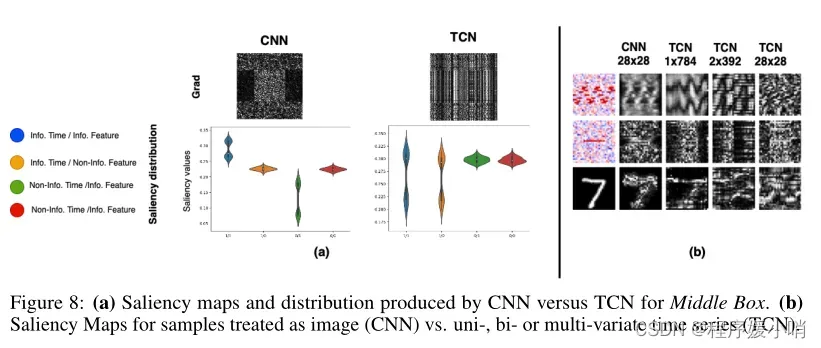
Figure 8: (a) Saliency maps and distribution produced by CNN versus TCN for Middle Box. (b) Saliency Maps for samples treated as image (CNN) vs. uni-, bi- or multi-variate time series (TCN)

图8:(a) CNN与TCN为Middle Box制作的显著性地图和分布。(b)作为图像处理的样本(CNN)与单变量、双变量或多变量时间序列(TCN)的显著性图

7 Temporal Saliency Rescaling

From the results presented in previous sections, we conclude that most saliency methods identify informative time steps successfully while they fail in identifying feature importance in those time steps.

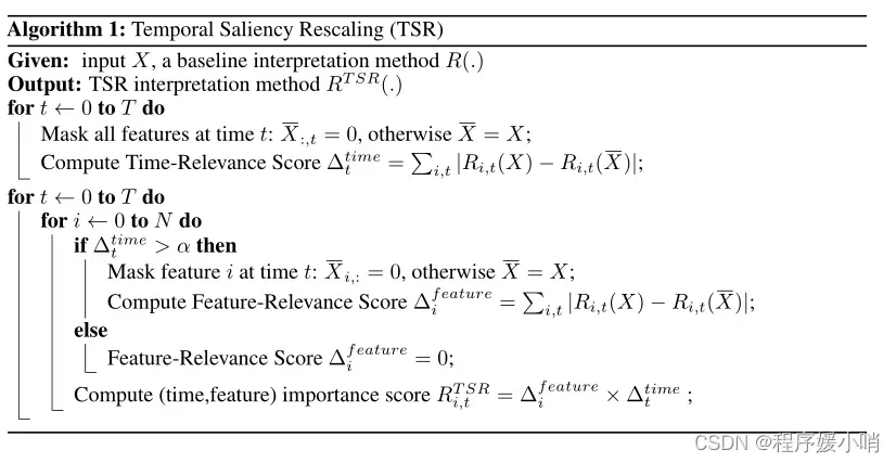
In this section, we propose a method that can be used on top of any generic interpretation method to boost its performance in time series applications. The key idea is to decouple the (time,feature) importance scores to time and feature relevance scores using a two-step procedure called Temporal Saliency Rescaling (TSR). In the first step, we calculate the time-relevance score for each time by computing the total change in saliency values if that time step is masked. Based on our experiments presented in the last sections, many existing interpretation methods would provide reliable timerelevance scores. In the second step, in each time-step whose time-relevance score is above a certain threshold α, we compute the feature-relevance score for each feature by computing the total change in saliency values if that feature is masked. By choosing a proper value for α, the second step can be performed in a few highly-relevant time steps to reduce the overall computational complexity of the method. Then, the final (time, feature) importance score is the product of associated time and feature relevance scores. The method is formally presented in Algorithm 1.

从前几节给出的结果中，我们得出结论，大多数显著性方法都成功地识别了信息时间步骤，而它们无法识别这些时间步骤中的特征重要性。

在本节中，我们提出了一种可以用于任何通用解释方法之上的方法，以提高时间序列应用程序中的性能。
关键的思想是使用两步程序将(时间，特征)重要性得分与时间和特征相关性得分解耦，称为时间显著性重新缩放(TSR)。
在第一步中，我们**通过计算显著性值的总变化(如果该时间步长被掩盖)来计算每次的时间相关性得分。**基于我们在上一节中提出的实验，许多现有的解释方法将提供可靠的时间相关性分数。
在第二步中，在每个时间步中，其时间相关性得分高于某个阈值α，我们通过计算显著性值的总变化来计算每个特征的特征相关性得分，如果该特征被掩盖。通过为α选择一个合适的值，
第二步可以在几个高度相关的时间步内执行，以降低方法的整体计算复杂度。然后，最终的(时间，特征)重要性得分是相关时间和特征相关性得分的乘积。算法1给出了该方法的形式。

Figure 5 shows updated saliency maps when applying TSR on the same examples in Figures 4.
There is a definite improvement in saliency quality across different architectures and interpretability methods except for SmoothGrad; this is probably because SmoothGrad adds noise to gradients, and using a noisy gradient as a baseline may not be appropriate. Table 1 shows the performance of TSR with simple Gradient compared to some standard saliency method on the benchmark metrics described in Section 4. TSR + Grad outpreforms other methods on all metrics.

图5显示了在图4中的相同示例上应用TSR时更新的显著性图。
除了SmoothGrad之外，不同架构和可解释性方法的显著性质量都有了明显的提高;这可能是因为SmoothGrad在渐变中添加了噪声，使用噪声梯度作为基线可能不合适。表1显示了在第4节中描述的基准指标上，与一些标准显著性方法相比，使用简单梯度的TSR的性能。TSR + Grad在所有指标上都优于其他方法。

The proposed rescaling approach improves the ability of saliency methods to capture feature importance over time but significantly increases the computational cost of producing a saliency map. Other approaches [14, 10] have relied on a similar trade-off between interpretability and computational complexity. In the supplementary material, we show the effect of applying temporal saliency rescaling on other datasets and provide possible optimizations.

**所提出的重新缩放方法提高了显著性方法随时间捕获特征重要性的能力，但显着增加了生成显著性图的计算成本。**其他方法[14,10]依赖于可解释性和计算复杂性之间的类似权衡。在补充材料中，我们展示了应用时间显著性重新缩放对其他数据集的影响，并提供了可能的优化。

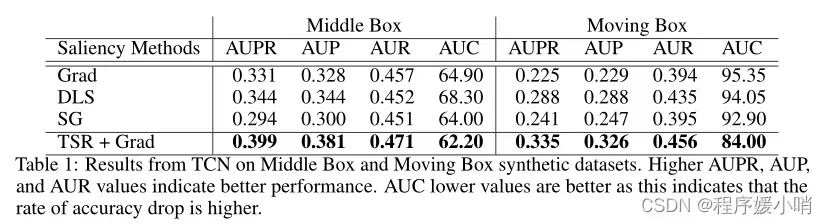
Table 1: Results from TCN on Middle Box and Moving Box synthetic datasets. Higher AUPR, AUP , and AUR values indicate better performance. AUC lower values are better as this indicates that the rate of accuracy drop is higher.

表1:TCN在中间盒子和移动盒子合成数据集上的结果。AUPR、AUP和AUR值越高，性能越好。AUC值越低越好，因为这表明准确率下降的速率越高。

8 Summary and Conclusion

In this work, we have studied deep learning interpretation methods when applied to multivariate time series data on various neural network architectures. To quantify the performance of each (interpretation method, architecture) pair, we have created a comprehensive synthetic benchmark where positions of informative features are known. We measure the quality of the generated interpretation by calculating the degradation of the trained model accuracy when inferred salient features are masked.These feature sets are then used to calculate the precision and recall for each pair.

在这项工作中，我们研究了将深度学习解释方法应用于各种神经网络架构上的多元时间序列数据。为了量化每个(解释方法、体系结构)对的性能，我们创建了一个综合的综合基准，其中信息特征的位置是已知的。当推断的显著特征被掩盖时，我们通过计算训练模型精度的退化来衡量生成解释的质量。然后使用这些特征集来计算每对的精度和召回率。

Interestingly, we have found that commonly-used saliency methods, including both gradient-based, and perturbation-based methods, fail to produce high-quality interpretations when applied to multivariate time series data. However, they can produce accurate maps when multivariate time series are represented as either images or univariate time series. That is, when temporal and feature domains are combined in a multivariate time series, saliency methods break down in general. The exact mathematical mechanism underlying this result is an open question. Consequently, there is no clear distinction in performance between different interpretability methods on multiple evaluation metrics when applied to multivariate time series, and in many cases, the performance is similar to random saliency. Through experiments, we observe that methods generally identify salient time steps but cannot distinguish important vs. non-important features within a given time step. Building on this observation, we then propose a two-step temporal saliency rescaling approach to adapt existing saliency methods to time series data. This approach has led to substantial improvements in the quality of saliency maps produced by different methods.

有趣的是，我们发现常用的显著性方法，包括基于梯度的方法和基于扰动的方法，在应用于多元时间序列数据时无法产生高质量的解释。然而，当多元时间序列被表示为图像或单变量时间序列时，它们可以生成精确的maps。
也就是说，当时间域和特征域在多元时间序列中结合时，显着性方法通常会失效。
这一结果背后的确切数学机制是一个悬而未决的问题。
因此，当应用于多元时间序列时，不同的可解释性方法在多个评价指标上的性能没有明显的区别，在许多情况下，性能类似于随机显著性。
通过实验，我们观察到，方法通常识别显著的时间步长，但不能在给定的时间步长内区分重要和不重要的特征。在此观察的基础上，我们提出了一种两步时间显著性重新缩放方法，使现有的显著性方法适应时间序列数据。这种方法使得不同方法生成的显著性图的质量有了实质性的改进。

9 Broader Impact

The challenge presented by meaningful interpretation of Deep Neural Networks (DNNs) is a technical barrier preventing their serious adoption by practitioners in fields such as Neuroscience, Medicine, and Finance [40, 41]. Accurate DNNs are not, by themselves, sufficient to be used routinely in high stakes applications such as healthcare. For example, in clinical research, one might like to ask, “why did you predict this person as more likely to develop a certain disease?” Our work aims to answer such questions. Many critical applications involve time series data, e.g., electronic health records, functional Magnetic Resonance Imaging (fMRI) data, and market data; nevertheless, the majority of research on interpretability focuses on vision and language tasks. Our work aims to interpret DNNs applied to time series data.

对深度神经网络(dnn)进行有意义的解释所带来的挑战是一个技术障碍，阻碍了神经科学、医学和金融等领域的从业者认真采用它们[40,41]。精确的dnn本身并不足以常规用于医疗等高风险应用。例如，在临床研究中，有人可能会问，“为什么你预测这个人更容易患上某种疾病?”我们的工作旨在回答这些问题。许多关键应用涉及时间序列数据，例如电子健康记录、功能磁共振成像(fMRI)数据和市场数据;然而，大多数关于可解释性的研究都集中在视觉和语言任务上。我们的工作旨在解释应用于时间序列数据的dnn。

Having interpretable DNNs has many positive outcomes. It will help increase the transparency of these models and ease their applications in a variety of research areas. Understanding how a model makes its decisions can help guide modifications to the model to produce better and fairer results. Critically, failure to provide faithful interpretations is a severe negative outcome. Having no interpretation at all is, in many situations, better than trusting an incorrect interpretation. Therefore, we believe this study can lead to significant positive and broad impacts in different applications.

拥有可解释的dnn有许多积极的结果。它将有助于提高这些模型的透明度，并简化它们在各种研究领域的应用。了解模型如何做出决策有助于指导对模型的修改，从而产生更好、更公平的结果。重要的是，未能提供忠实的解释是一个严重的负面结果。在许多情况下，完全没有解释比相信一个不正确的解释要好。因此，我们相信这项研究可以在不同的应用中产生显著的积极和广泛的影响。