使用PyTorch构建神经网络，并使用thop计算参数和FLOPs

文章目录

- 使用PyTorch构建神经网络，并使用thop计算参数和FLOPs
- - FLOPs和FLOPS区别
  - 使用PyTorch搭建神经网络
  - - 整体代码
    - 1. 导入必要的库
    - 2. 定义神经网络模型
    - 3. 打印网络结构
    - 4. 计算网络FLOPs和参数数量
    - 5. 结果如下
    - 手动计算params
    - 手动计算FLOPs
    - 注意

使用PyTorch构建神经网络，并使用thop计算参数和FLOPs

FLOPs和FLOPS区别

FLOPs（floating point operations）是指浮点运算次数，通常用来评估一个计算机算法或者模型的计算复杂度。在机器学习中，FLOPs通常用来衡量神经网络的计算复杂度，因为神经网络的计算主要由矩阵乘法和卷积操作组成，而这些操作都可以转化为浮点运算次数的形式进行计算。

FLOPS（floating point operations per second）是指每秒钟可以执行的浮点运算次数，通常用来评估一个计算机系统的计算能力。在机器学习中，FLOPS也可以用来衡量计算机系统的性能，因为神经网络的训练和推断需要大量的浮点运算，计算机系统的FLOPS越高，就越能够快速地完成神经网络的计算任务。

需要注意的是，FLOPs和FLOPS都是衡量计算复杂度和计算能力的指标，但它们的单位不同，FLOPs的单位是次，而FLOPS的单位是次/秒。FLOPs和FLOPS是两个不同的概念，FLOPs是指浮点运算次数，而FLOPS是指每秒钟可以执行的浮点运算次数。在实际应用中，我们通常会同时考虑这两个指标，以评估计算机算法或者模型在不同的计算机系统上的表现。

使用PyTorch搭建神经网络

整体代码

import torch
import torch.nn as nn
from torchsummary import summary
from thop import profile, clever_format


device = torch.device("cuda" if torch.cuda.is_available() else "cpu")
class MyNet(nn.Module):
    def __init__(self, *args, **kwargs) -> None:
        super().__init__(*args, **kwargs)
        self.conv1 = nn.Conv2d(3, 64, kernel_size=3, stride=1, padding=1)
        self.relu1 = nn.ReLU(inplace=True)
        self.conv2 = nn.Conv2d(64, 64, kernel_size=3, stride=1, padding=1)
        self.relu2 = nn.ReLU(inplace=True)
        self.maxpool = nn.MaxPool2d(kernel_size=2, stride=2)
        self.conv3 = nn.Conv2d(64, 128, kernel_size=3, stride=1, padding=1)
        self.relu3 = nn.ReLU(inplace=True)
        self.conv4 = nn.Conv2d(128, 128, kernel_size=3, stride=1, padding=1)
        self.relu4 = nn.ReLU(inplace=True)
        self.fc1 = nn.Linear(128*8*8, 1024)
        self.relu5 = nn.ReLU(inplace=True)
        self.fc2 = nn.Linear(1024, 10)

    def forward(self, x):
        x = self.conv1(x)
        x = self.relu1(x)
        x = self.conv2(x)
        x = self.relu2(x)
        x = self.maxpool(x)
        x = self.conv3(x)
        x = self.relu3(x)
        x = self.conv4(x)
        x = self.relu4(x)
        x = x.view(-1, 128*8*8)
        x = self.fc1(x)
        x = self.relu5(x)
        x = self.fc2(x)
        return x
    
net = MyNet().to(device)
input_shape = (3, 224, 224)
summary(net, input_shape)

input_tensor = torch.randn(1, *input_shape).to(device)
flops, params = profile(net, inputs=(input_tensor,))
flops, params = clever_format([flops, params], "%.3f")
print("FLOPs: %s" %(flops))
print("params: %s" %(params))

这段代码是一个使用PyTorch实现的卷积神经网络。下面是一步一步的教程：

1. 导入必要的库

import torch
import torch.nn as nn
from torchsummary import summary
from thop import profile, clever_format

其中，torch是PyTorch深度学习框架的核心库，torch.nn是PyTorch中神经网络相关的模块，torchsummary是用于打印网络结构的库，thop是用于计算网络FLOPs和参数数量的库。

2. 定义神经网络模型

class MyNet(nn.Module):
    def __init__(self, *args, **kwargs) -> None:
        super().__init__(*args, **kwargs)
        self.conv1 = nn.Conv2d(3, 64, kernel_size=3, stride=1, padding=1)
        self.relu1 = nn.ReLU(inplace=True)
        self.conv2 = nn.Conv2d(64, 64, kernel_size=3, stride=1, padding=1)
        self.relu2 = nn.ReLU(inplace=True)
        self.maxpool = nn.MaxPool2d(kernel_size=2, stride=2)
        self.conv3 = nn.Conv2d(64, 128, kernel_size=3, stride=1, padding=1)
        self.relu3 = nn.ReLU(inplace=True)
        self.conv4 = nn.Conv2d(128, 128, kernel_size=3, stride=1, padding=1)
        self.relu4 = nn.ReLU(inplace=True)
        self.fc1 = nn.Linear(128*8*8, 1024)
        self.relu5 = nn.ReLU(inplace=True)
        self.fc2 = nn.Linear(1024, 10)

    def forward(self, x):
        x = self.conv1(x)
        x = self.relu1(x)
        x = self.conv2(x)
        x = self.relu2(x)
        x = self.maxpool(x)
        x = self.conv3(x)
        x = self.relu3(x)
        x = self.conv4(x)
        x = self.relu4(x)
        x = x.view(-1, 128*8*8)
        x = self.fc1(x)
        x = self.relu5(x)
        x = self.fc2(x)
        return x

这个网络模型包括了4个卷积层、2个全连接层和ReLU激活函数。其中，nn.Conv2d是PyTorch中的二维卷积层，nn.ReLU是ReLU激活函数层，nn.MaxPool2d是最大池化层，nn.Linear是全连接层。这个模型的输入是一个3通道、224×224大小的图像，输出是一个10维的向量，分别表示输入图像属于10个不同的类别的概率。

3. 打印网络结构

device = torch.device("cuda" if torch.cuda.is_available() else "cpu")
net = MyNet().to(device)
input_shape = (3, 224, 224)
summary(net, input_shape)

这里我们首先根据设备是否支持CUDA来选择使用CPU或GPU，然后将模型实例化为net并将其放到设备上。接着，我们定义输入图像的形状为(3, 224, 224)，然后使用summary函数打印网络的结构信息，包括每一层的输入和输出形状、参数数量等。

4. 计算网络FLOPs和参数数量

input_tensor = torch.randn(1, *input_shape).to(device)
flops, params = profile(net, inputs=(input_tensor,))
flops, params = clever_format([flops, params], "%.3f")
print("FLOPs: %s" %(flops))
print("params: %s" %(params))

这里我们使用随机生成的输入图像进行前向传播，然后使用profile函数计算网络的FLOPs和参数数量。inputs参数接受一个元组，其中包含了网络的输入，这里我们将随机生成的输入图像封装成一个元组传入。计算完成后，使用clever_format函数将FLOPs和参数数量格式化成易读的字符串形式，最后打印出来。

5. 结果如下

----------------------------------------------------------------
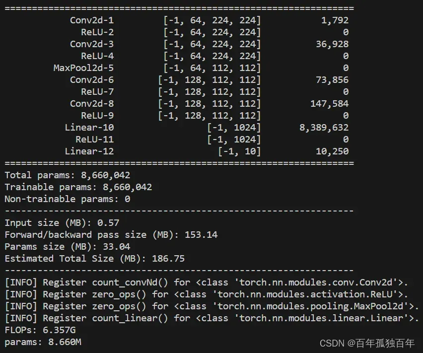
        Layer (type)               Output Shape         Param #
================================================================
            Conv2d-1         [-1, 64, 224, 224]           1,792
              ReLU-2         [-1, 64, 224, 224]               0
            Conv2d-3         [-1, 64, 224, 224]          36,928
              ReLU-4         [-1, 64, 224, 224]               0
         MaxPool2d-5         [-1, 64, 112, 112]               0
            Conv2d-6        [-1, 128, 112, 112]          73,856
              ReLU-7        [-1, 128, 112, 112]               0
            Conv2d-8        [-1, 128, 112, 112]         147,584
              ReLU-9        [-1, 128, 112, 112]               0
           Linear-10                 [-1, 1024]       8,389,632
             ReLU-11                 [-1, 1024]               0
           Linear-12                   [-1, 10]          10,250
================================================================
Total params: 8,660,042
Trainable params: 8,660,042
Non-trainable params: 0
----------------------------------------------------------------
Input size (MB): 0.57
Forward/backward pass size (MB): 153.14
Params size (MB): 33.04
Estimated Total Size (MB): 186.75
----------------------------------------------------------------
[INFO] Register count_convNd() for <class 'torch.nn.modules.conv.Conv2d'>.
[INFO] Register zero_ops() for <class 'torch.nn.modules.activation.ReLU'>.
[INFO] Register zero_ops() for <class 'torch.nn.modules.pooling.MaxPool2d'>.
[INFO] Register count_linear() for <class 'torch.nn.modules.linear.Linear'>.
FLOPs: 6.357G
params: 8.660M

这段代码定义了一个简单的卷积神经网络模型，然后使用thop库计算模型的FLOPs（浮点运算次数）和参数数量。

手动计算params

好的，这里是每一层的参数计算公式：

Conv2d层：参数数量 = (输入通道数 x 卷积核高度 x 卷积核宽度 x 输出通道数) + 输出通道数
Linear层：参数数量 = 输入大小 x 输出大小 + 输出大小
没有参数的层（如ReLU和MaxPool）不需要计算参数数量。

具体来说，在这个神经网络中，每一层的参数计算公式和参数数量如下：

Conv2d-1：(3 x 3 x 3 x 64) + 64 = 1,792
ReLU-2：没有参数
Conv2d-3：(3 x 3 x 64 x 64) + 64 = 36,928
ReLU-4：没有参数
MaxPool2d-5：没有参数
Conv2d-6：(3 x 3 x 64 x 128) + 128 = 73,856
ReLU-7：没有参数
Conv2d-8：(3 x 3 x 128 x 128) + 128 = 147,584
ReLU-9：没有参数
Linear-10：(128 x 56 x 56 x 1024) + 1024 = 8,389,632
ReLU-11：没有参数
Linear-12：(1024 x 10) + 10 = 10,250

总参数数为8,660,042个。

手动计算FLOPs

Thop（PyTorch-OpCounter）是一个用于计算PyTorch模型浮点运算量（FLOPs）的库，它可以自动计算模型中每个操作的FLOPs，包括卷积层、池化层、全连接层等。

在Thop中，FLOPs的计算基于每个操作的输入张量大小、输出张量大小以及操作的参数数量。具体地，对于一个卷积层，FLOPs的计算公式为：

使用PyTorch构建神经网络，并使用thop计算参数和FLOPs

其中，使用PyTorch构建神经网络，并使用thop计算参数和FLOPs 是卷积核大小，是输入通道数，是输出通道数，和是输出特征图的高度和宽度，是步幅。这个公式中的常数2表示每个卷积操作需要2次乘法（一个是卷积核和输入的卷积，另一个是卷积结果和偏置的加法），因此需要乘以2。

对于其他层类型，Thop使用不同的公式计算FLOPs。例如，对于全连接层，FLOPs的计算公式为：

使用PyTorch构建神经网络，并使用thop计算参数和FLOPs

其中，使用PyTorch构建神经网络，并使用thop计算参数和FLOPs 和分别是输入和输出的特征数量。

通过使用Thop库，您可以方便地计算模型的总体FLOPs，以评估模型的计算复杂度和性能。

池化层和ReLU层的计算复杂度相对简单，可以用以下公式进行计算：

对于池化层，假设输入特征图大小为使用PyTorch构建神经网络，并使用thop计算参数和FLOPs ，池化尺寸为，步幅为，则池化层的FLOPs计算公式为：

使用PyTorch构建神经网络，并使用thop计算参数和FLOPs

其中，使用PyTorch构建神经网络，并使用thop计算参数和FLOPs ，，是输入特征图的通道数。这个公式中的常数表示每个池化操作需要次取最大值。

对于ReLU层，假设输入特征图大小为使用PyTorch构建神经网络，并使用thop计算参数和FLOPs ，ReLU层的计算量可以近似为：

使用PyTorch构建神经网络，并使用thop计算参数和FLOPs

这是因为ReLU激活函数的计算本身非常简单，只需要比较输入数据与0，然后保留大于0的值即可，因此单个ReLU激活函数的计算量可以视为常数。

需要注意的是，这些公式只是近似计算，实际的计算复杂度可能会因为不同实现方式、硬件平台等因素而有所不同。对于更准确的计算，可以使用一些工具库（如Thop）来进行计算。

为了解释为什么得到的FLOPs是6.357G，我们需要逐层分析模型中的计算量。以下是计算步骤（不考虑relu和pool层）：

conv1: (3 × 3 × 3) × 64 × 224 × 224 = 86,704,128 FLOPs
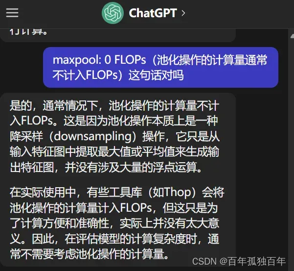
relu1: 0 FLOPs（ReLU激活函数的计算量通常不计入FLOPs） # 3211264
conv2: (3 × 3 × 64) × 64 × 224 × 224 = 1,849,688,064 FLOPs
relu2: 0 FLOPs # 3211264
maxpool: 0 FLOPs（池化操作的计算量通常不计入FLOPs） # 32111254
conv3: (3 × 3 × 64) × 128 × 112 × 112 = 924,844,032 FLOPs
relu3: 0 FLOPs 128112112=1605632
conv4: (3 × 3 × 128) × 128 × 112 × 112 = 1,849,688,064 FLOPs
relu4: 0 FLOPs # 1605632
fc1: 128 × 8 × 8 × 1024 = 8,388,608 FLOPs
relu5: 0 FLOPs # 这个计算FLOPs我懵了。按20480吧
fc2: 1024 × 10 = 10,240 FLOPs

将各层的FLOPs相加，得到总的FLOPs：

86,704,128 + 1,849,688,064 + 924,844,032 + 1,849,688,064 + 8,388,608 + 10240 = 4,719,323,136 FLOPs

然后将FLOPs转换为GigaFLOPs（10^9 FLOPs）：

4,719,323,136 / 10^9 ≈ 4.719 GigaFLOPs

4.719远远不等于6.357啊！

如果按照全部乘以2，又变成9点多了，又远远超过6.357了。

听说profile算出来的FLOPs也需要乘以2。按照这么想的话，咱们手动计算的结果不乘2应该和thop计算出来的相当。但是结果相当打脸，远远不等。

所以relu层和pool层肯定带入FLOPs了。

加粗样式

恩。。。怎么说呢

注意

显然，结果与代码中计算得到的6.357G不符。这就有点奇怪了？

消失的1.638G去哪里了？

就是把relu层和池化层的全部加上也不够啊！加上relu和池化层的结果如下。

86,704,128 + 3211264 + 1,849,688,064 + 3211254 + 32111254 + 924,844,032 + 1605632 + 1,849,688,064 + 1605632 + 8,388,608 + 10240 + 10240 = 4,761,078,412 FLOPs

relu和maxpool再怎么套公式，也算不上去了，加不了那么多。算了。。。。以后有时间再慢慢算吧，谁和thop计算的一样可以留言公式，我去学习一下。

G去哪里了？

就是把relu层和池化层的全部加上也不够啊！加上relu和池化层的结果如下。

86,704,128 + 3211264 + 1,849,688,064 + 3211254 + 32111254 + 924,844,032 + 1605632 + 1,849,688,064 + 1605632 + 8,388,608 + 10240 + 10240 = 4,761,078,412 FLOPs

relu和maxpool再怎么套公式，也算不上去了，加不了那么多。算了。。。。以后有时间再慢慢算吧，谁和thop计算的一样可以留言公式，我去学习一下。

**可能原因：**这可能是因为thop库在计算FLOPs时考虑了一些其他因素，relu和pool也计算进去了，而且占比还挺多，莫名增加了1.638G。因此，实际计算得到的FLOPs可能会与手动计算的结果有所不同。即使如此，手动计算的结果可以帮助我们理解FLOPs~~的大致数量级。~~

文章出处登录后可见！

已经登录？立即刷新

使用PyTorch构建神经网络，并使用thop计算参数和FLOPs

文章目录

使用PyTorch构建神经网络，并使用thop计算参数和FLOPs

FLOPs和FLOPS区别

使用PyTorch搭建神经网络

整体代码

1. 导入必要的库

2. 定义神经网络模型

3. 打印网络结构

4. 计算网络FLOPs和参数数量

5. 结果如下

手动计算params

手动计算FLOPs

注意

相关推荐