1. 引言
今天我们将重点讨论霍夫变换,这是一种非常经典的线检测的算法,通过将图像中的点映射到参数空间中的线来实现。霍夫变换可以检测任何方向的线,并且可以在具有大量噪声的图像中很好地工作。
闲话少说,我们直接开始吧!
2. 基础知识
为了理解霍夫变换的工作原理,首先我们需要了解直线是如何在极坐标系中定义的。直线由ρ(距原点的垂直距离)和θ(垂直线与轴线的夹角)来描述,如下图所:
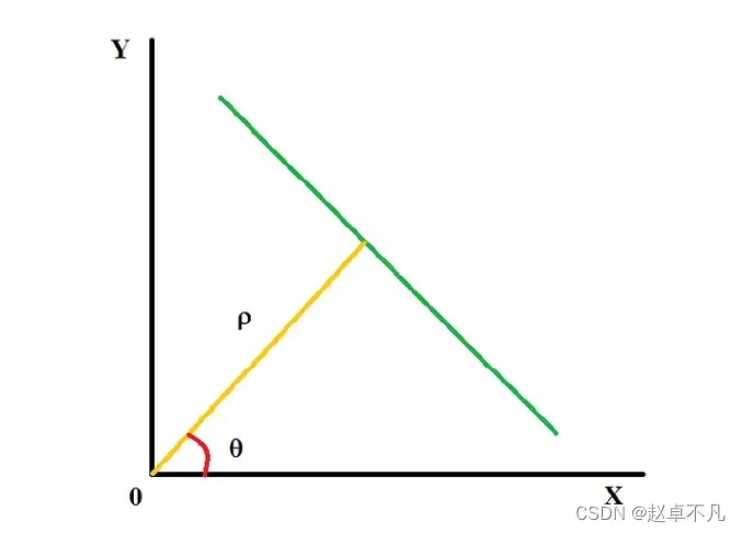
因此,该直线的方程式为:
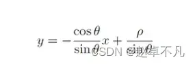
我们可以将其转化下表述形式,得到如下公式:
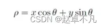
从上面的方程中,我们可以看出,所有具有相同ρ和θ值的点构成一条直线。我们算法的基础是针对θ的所有可能值计算图像中每个点的ρ值。
3. 算法原理
霍夫变换的处理步骤如下:
1)首先我们创建一个参数空间(又叫做霍夫空间)。参数空间是ρ和θ的二维矩阵,其中θ的范围在0–180之间。
2)使用诸如Canny边缘之类的边缘检测算法检测图像的边缘之后运行该算法。值为255的像素被认为是边缘。
3)接着我们逐像素扫描图像以找到这些边缘像素,并通过使用从0到180的θ值来计算每个像素的ρ。对于同一直线上的像素,θ和rho的值将是相同的。我们在霍夫空间中以1的权重对其投票。
4)最后,投票超过一定阈值的ρ和θ的值被视为直线。
代码处理过程如下:
def hough(img):
    # Create a parameter space
    # Here we use a dictionary
    H=dict()
    # We check for pixels in image which have value more than 0(not black)
    co=np.where(img>0)
    co=np.array(co).T
    for point in co:
        for t in range(180):
            # Compute rho for theta 0-180
            d=point[0]*np.sin(np.deg2rad(t))+point[1]*np.cos(np.deg2rad(t))
            d=int(d)
            # Compare with the extreme cases for image
            if d<int(np.ceil(np.sqrt(np.square(img.shape[0]) + np.square(img.shape[1])))):
                if (d,t) in H:
                    # Upvote
                    H[(d,t)] += 1
                else:
					# Create a new vote
                    H[(d,t)] = 1
    return H
4. 算法应用
在本文中,我们将检测图像中对象(书籍)的角点。这似乎是一项简单的任务,然而,它将让我们深入了解使用霍夫变换检测直线的过程。
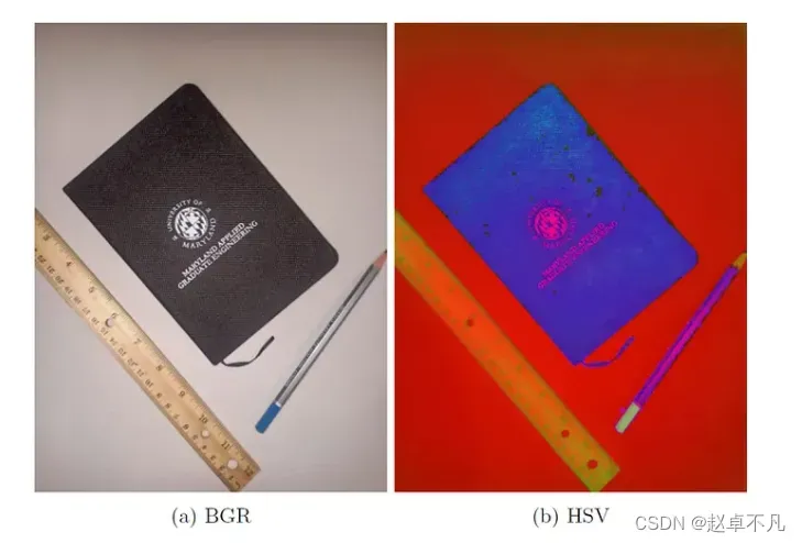
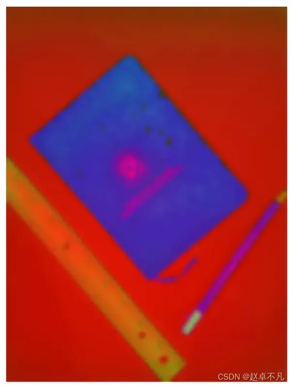
4.1 彩色图到HSV空间
由于直接RGB图像做这项任务略有难度,我们不妨将该图像转换为HSV颜色空间,以便在HSV范围内轻松获取我们的目标。
核心代码如下:
img = cv2.imread("book.jpeg")
scale_percent = 30 # percent of original size
width = int(img.shape[1] * scale_percent / 100)
height = int(img.shape[0] * scale_percent / 100)
dim = (width, height)
# resize image
img = cv2.resize(img, dim, interpolation = cv2.INTER_AREA)
hsv = cv2.cvtColor(img, cv2.COLOR_BGR2HSV)
得到结果如下所示:
4.2 高斯模糊
我们应用高斯模糊来平滑图像中由于噪声而产生的粗糙边缘,进而可以突出我们图像中的目标,代码如下:
# Apply gaussian blur to he mask
blur = cv2.GaussianBlur(hsv, (9, 9), 3)
结果如下所示:
4.3 二值化和腐蚀操作
接着我们使用inRange函数来得到二值化图像。这使我们能够摆脱图像中其他周围的物体。代码如下:
# Define the color range for the ball (in HSV format)
lower_color = np.array([0, 0, 24],np.uint8)
upper_color = np.array([179, 255, 73],np.uint8)
# Define the kernel size for the morphological operations
kernel_size = 7
# Create a mask for the ball color using cv2.inRange()
mask = cv2.inRange(blur, lower_color, upper_color)
得到结果如下:
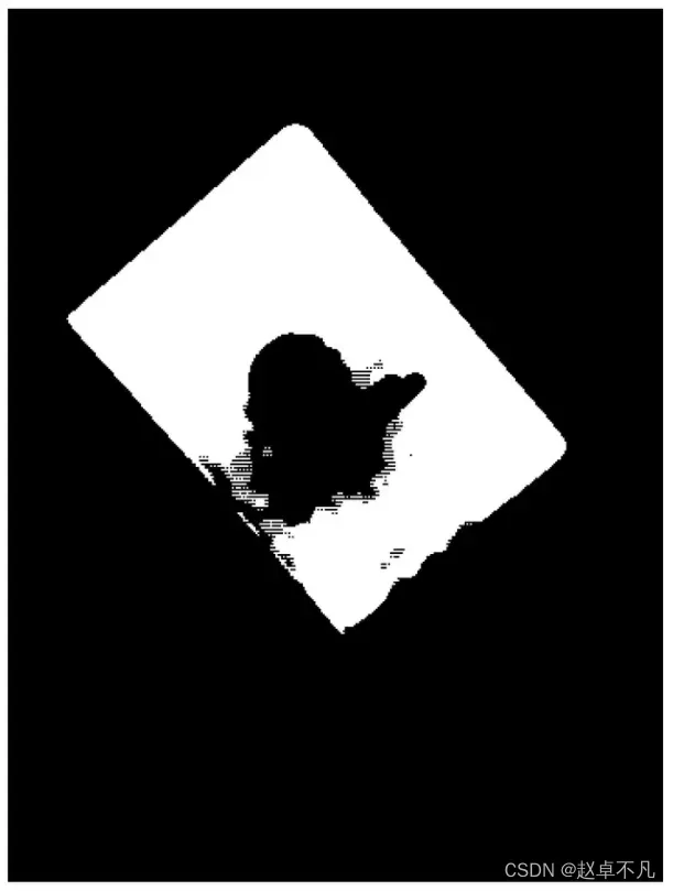
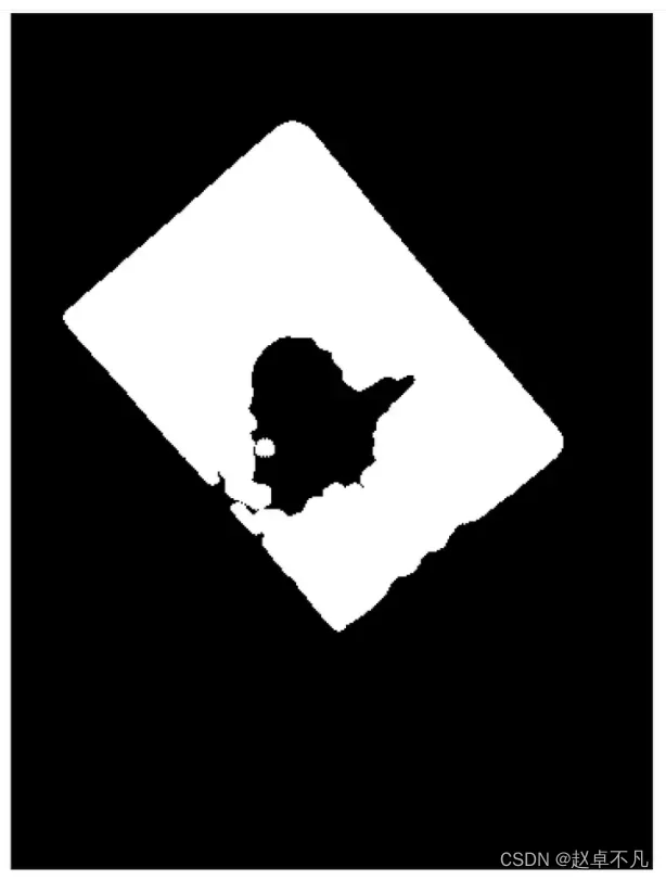
我们观察上图,存在或多或少的缝隙,我们不妨使用腐蚀操作来填补这些缝隙。代码如下:
# Apply morphological operations to the mask to fill in gaps
kernel = cv2.getStructuringElement(cv2.MORPH_ELLIPSE, (kernel_size, kernel_size))
mask = cv2.dilate(mask, kernel,iterations=1)
结果如下:
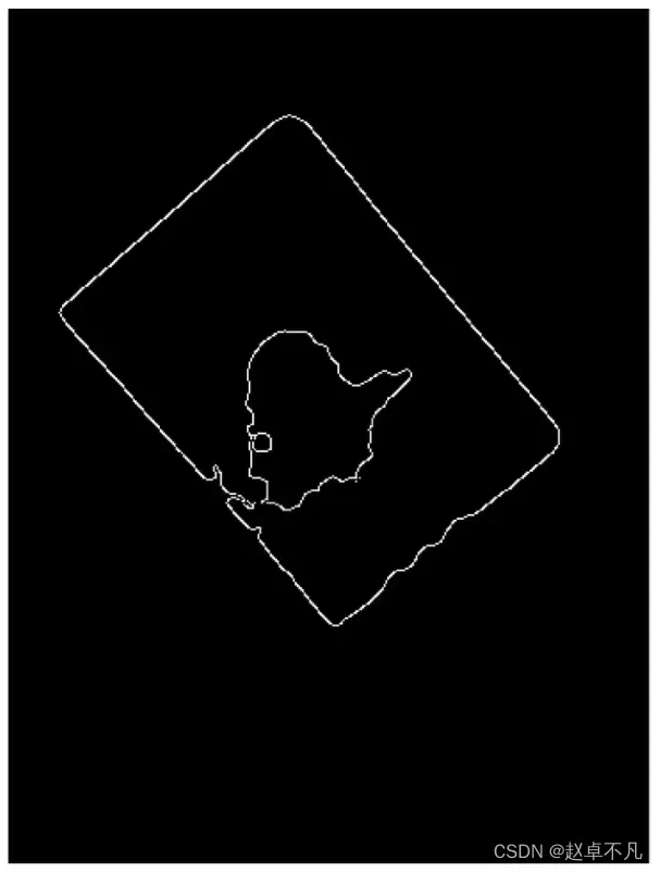
4.4 边缘检测
边缘检测canny主要用于检测边缘。这主要是因为目标和周围背景之间的高对比度。代码如下:
#  Use canny edges to get the edges of the image mask
edges = cv2.Canny(mask,200, 240, apertureSize=3)
结果如下图所示:
4.5 霍夫变换
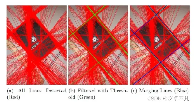
当我们进行canny边缘检测时,我们得到了很多边缘。因此,当我们运行霍夫算法时,这些边为同一条边贡献了许多条候选线。为了解决这个问题,我们对霍夫空间中ρ和θ的相邻值进行聚类,并对它们的值进行平均,得到它们的上投票数之和。这导致了描绘相同边缘的线条的合并,代码如下:
# Get the hough space, sort and select to 20 values
hough_space = dict(sorted(hough(edges).items(), key=lambda item: item[1],reverse=True)[:20])
# Sort the hough space w.r.t rho and theta
sorted_hough_space_unfiltered = dict(sorted(hough_space.items()))
# Get the unique rhoand theta values
unique_=unique(sorted_hough_space_unfiltered)
# Sort according to value and get the top 4 lines
unique_=dict(sorted(unique_.items(), key=lambda item: item[1],reverse=True)[:4])
得到结果如下:
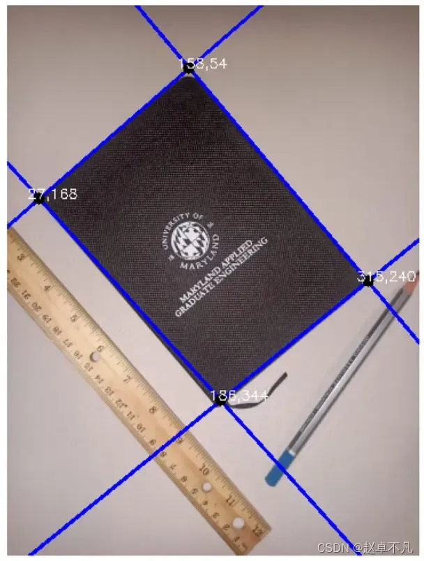
4.6 计算角点
根据在霍夫空间中获得的直线,我们可以使用线性代数对其进行角点求解。这可以求出我们两条直线的交叉点,也就是书的角点,代码如下:
# Create combinations of lines
line_combinations = list(combinations(unique_.items(), 2))

intersection=[]
filter_int=[]
for (key1, value1), (key2, value2) in line_combinations:
    try:
	# Solve point of intersection of two lines
        intersection.append(intersection_point(key1[0],np.deg2rad(key1[1]), key2[0],np.deg2rad(key2[1])))
    except:
        print("Singular Matrix")

for x,y in intersection:
    if x>0 and y>0:
		# Get the valid cartesan co ordinates
        cv2.circle(img, (x, y), 5, (0, 0, 0), -1)
        cv2.putText(img, '{},{}'.format(x,y), (x-10, y), cv2.FONT_HERSHEY_SIMPLEX, 0.4, (255, 255, 255), 1)
        filter_int.append([x,y])
最终输出如下图所示:
5. 总结
尽管该算法现已集成在各种各样的图像处理库,但本文通过自己实现它,我们可以深入了解在创建如此复杂的算法时所面临的挑战和局限性。
嗯嗯,您学废了嘛?
代码链接:戳我
文章出处登录后可见!