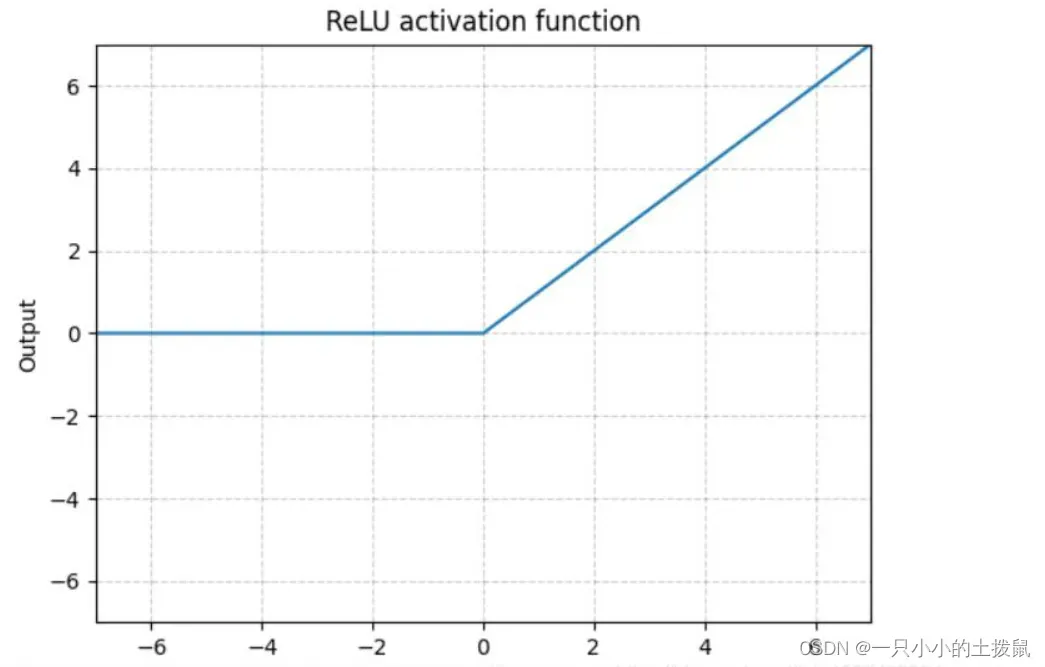
1、torch.nn.ReLU()
数学表达式
![]()
ReLU的函数图示如下:
优点:
(1)收敛速度比 sigmoid 和 tanh 快;(梯度不会饱和,解决了梯度消失问题)
(2)计算复杂度低,不需要进行指数运算
缺点:
(1)ReLu的输出不是zero-centered;
(2)Dead ReLU Problem(神经元坏死现象):某些神经元可能永远不会被激活,导致相应参数不会被更新(在负数部分,梯度为0)。产生这种现象的两个原因:参数初始化问题;learning rate太高导致在训练过程中参数更新太大。解决办法:采用Xavier初始化方法;以及避免将learning rate设置太大或使用adagrad等自动调节learning rate的算法。
(3)ReLu不会对数据做幅度压缩,所以数据的幅度会随着模型层数的增加不断扩张。
import torch
import torch.nn as nn
x = torch.randn(100, 10)
y = torch.randn(100, 30)

func = nn.ReLU()
output_x = func(x)
output_y = func(y)
print("Output size:", output_x.size())
print("Output size:", output_y.size())
# Output size: torch.Size([100, 10])
# Output size: torch.Size([100, 30])
print(x[0])
print(output_x[0])
# tensor([ 0.5594,  0.2387, -1.5372, -0.6874,  1.1714, -0.1458, -1.1784, -0.0802,-0.5905,  2.2499])
# tensor([0.5594, 0.2387, 0.0000, 0.0000, 1.1714, 0.0000, 0.0000, 0.0000, 0.0000,2.2499])

def relu(inX):
    return np.maximum(0,inX)
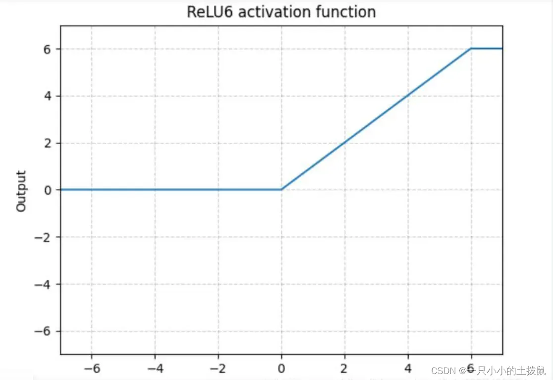
2、torch.nn.ReLU6()
数学表达式:
![]()
ReLU6是在ReLU的基础上,限制正值的上限6。
import torch
import torch.nn as nn
x = torch.randn(100, 10)* 10
y = torch.randn(100, 30)

func = nn.ReLU6()
output_x = func(x)
output_y = func(y)
print("Output size:", output_x.size())
print("Output size:", output_y.size())
# Output size: torch.Size([100, 10])
# Output size: torch.Size([100, 30])
print(x[0])
print(output_x[0])
# tensor([  8.1576,  11.7024,  -3.9226,  -2.6406,  11.0565, -16.3319,   7.0528, 0.8866,   0.6748,  -1.0607])
# tensor([6.0000, 6.0000, 0.0000, 0.0000, 6.0000, 0.0000, 6.0000, 0.8866, 0.6748, 0.0000])
3、torch.nn.LeakyReLU()
在标准的神经网络模型中,死亡梯度问题是常见的。为了避免这个问题,应用了leaky ReLU。Leaky ReLU允许一个小的非零梯度。
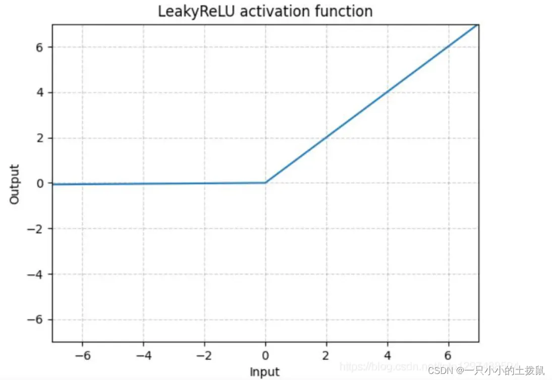
这里a是固定值,LeakyReLU的目的是为了避免激活函数不处理负值(小于0的部分梯度为0),通过使用negative slope,其使得网络可以在传递负值部分的梯度,让网络可以学习更多的信息
import torch
import torch.nn as nn
x = torch.randn(100, 10)
y = torch.randn(100, 30)

func = nn.LeakyReLU()
output_x = func(x)
output_y = func(y)
print("Output size:", output_x.size())
print("Output size:", output_y.size())
# Output size: torch.Size([100, 10])
# Output size: torch.Size([100, 30])
print(x[0])
print(output_x[0])
# tensor([ 1.0718, -0.3105, -0.2773,  1.8701,  0.2646, -0.2166,  1.1425,  1.1959,-2.7848, -0.2138])
# tensor([ 1.0718, -0.0031, -0.0028,  1.8701,  0.2646, -0.0022,  1.1425,  1.1959, -0.0278, -0.0021])
4、torch.nn.RReLU()
ReLU有很多变种, RReLU是Random ReLU的意思,在RReLU中,负值的斜率在训练中是随机的,在之后的测试中就变成了固定的了。RReLU的亮点在于,在训练环节中,a是从一个均匀的分布U(I,u)中随机抽取的数值。
数学表达式:

RReLU中的a是一个在一个给定的范围内随机抽取的值,这个值在测试环节就会固定下来。 对RReLU而言, a是一个在给定范围内的随机变量(训练), 在推理时保持不变。同LeakyReLU不同的是,RReLU的a是可以learnable的参数,而LeakyReLU的a是固定的。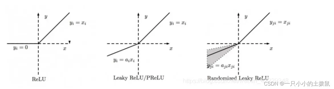
import torch
import torch.nn as nn
x = torch.randn(100, 10)
# torch.nn.RReLU(lower=0.125, upper=0.3333333333333333, inplace=False)
func = nn.RReLU(0.1, 0.3)
y = func(x)
print(x[0])
print(y[0])
# tensor([-0.4467,  0.3433,  0.0522,  0.5509,  1.7010, -0.1909,  0.6914, -0.6053, 0.5511, -1.9335])
# tensor([-0.0514,  0.3433,  0.0522,  0.5509,  1.7010, -0.0270,  0.6914, -0.1125, 0.5511, -0.5593])
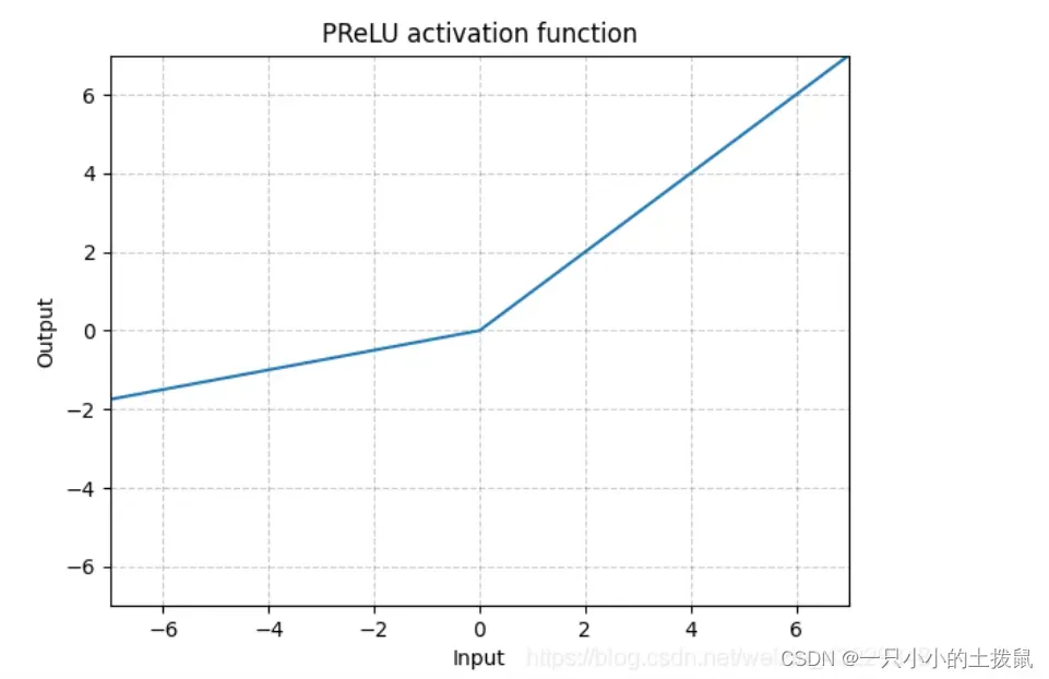
5、torch.nn.PReLU()
数学表达式:
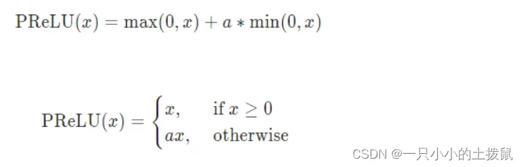
不同于RReLU的a可以是随机的,PReLU中的a就是一个learnable的参数。当不带参数调用时,nn.PReLU()在所有输入通道中使用单个参数a。如果使用nn.PReLU(nChannels)调用,则每个输入通道使用一个单独的a。n_channels表示第二维度数量。
import torch
import torch.nn as nn
x = torch.randn(100, 10)
# torch.nn.PReLU(num_parameters=1, init=0.25, device=None, dtype=None)
# num_parameters表示要学习的a的数量。尽管它接受一个int作为输入,但只有两个值是合法的:1,或者输入处的通道数量。默认值:1
# init:a的初始值,默认是0.25
func = nn.PReLU(10)
y = func(x)
print(x[0])
print(y[0])
# tensor([-0.5982, -0.5509, -0.7107, -0.4316, -0.5107,  0.4100, -1.3367,  1.5206, -2.4008, -1.1881])
# tensor([-0.1495, -0.1377, -0.1777, -0.1079, -0.1277,  0.4100, -0.3342,  1.5206, -0.6002, -0.2970], grad_fn=<SelectBackward>)
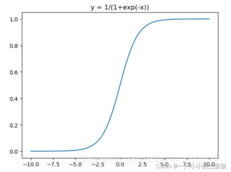
6、torch.nn.Sigmoid()
当我们将权值从神经网络的输入层传递到隐含层时,我们希望我们的模型能够捕获数据中呈现的所有非线性;因此,建议在神经网络的隐层中使用sigmoid函数。非线性函数有助于泛化数据集。用非线性函数计算函数的梯度比较容易。
sigmoid函数是一种特殊的非线性激活函数。sigmoid函数的输出总是限制在0和1之内;因此,它主要用于执行基于分类的任务。sigmoid函数的局限性之一是它可能会陷入局部极小值。这样做的好处是,它提供了属于这类的可能性。
数学表达式:

Sigmoid是将数据限制在0到1之间。而且,由于Sigmoid的最大的梯度为0.25,随着使用sigmoid的层越来越多,网络就变得很难收敛。
因此,对深度学习,ReLU及其变种被广泛使用避免收敛困难的问题。
优点:
(1)便于求导的平滑函数
(2)能压缩数据,保证数据幅度不会有问题
(3)适合用于前向传播
缺点:【梯度消失/幂运算耗时】
(1)容易出现梯度消失(gradient vanishing)的现象:当 激活函数 接近饱和区时,变化太缓慢,导数接近0,根据后向传递的数学依据是微积分求导的链式法则,当前导数需要之前各层导数的乘积,几个比较小的数相乘,导数结果很接近0,从而无法完成深层网络的训练。
(2)Sigmoid的输出不是0均值的:这会导致后层的神经元的输入是非0均值的信号,这会对梯度产生影响。以 f=sigmoid(wx+b)为例, 假设输入均为正数(或负数),那么对w的导数总是正数(或负数),这样在反向传播过程中要么都往正方向更新,要么都往负方向更新,导致有一种捆绑效果,使得收敛缓慢。
(3)幂运算相对耗时
import torch

x = torch.randn(100, 10)
y = torch.randn(100,30)
sig=nn.Sigmoid()
output_sigx = sig(x)
output_sigy = sig(y)
print("Output size:", output_sigx.size())
print("Output size:", output_sigy.size())
print(x[0])
print(output_sigx[0])
# Output size: torch.Size([100, 10])
# Output size: torch.Size([100, 30])
# tensor([ 0.4357, -1.5673, -0.8468,  0.0629, -1.2619, -0.2609, -0.3565,  0.5630, 1.8491,  0.3339])
# tensor([0.6072, 0.1726, 0.3001, 0.5157, 0.2206, 0.4351, 0.4118, 0.6372, 0.8640, 0.5827])

class Sigmoid(nn.Module):
	def __init__(self):
		super(Sigmoid, self).__init__()
	def forward(self, x):
		return 1./(1. + torch.exp(-x))

class Sigmoid(nn.Module):
	def __init__(self):
		super(Sigmoid, self).__init__()
	def forward(self, x):
		return F.sigmoid(x)
7、torch.nn.Tanh()
双曲正切函数是变换函数的另一种变体。它用于将信息从映射层转换到隐藏层。它通常用于神经网络模型的隐藏层之间。Tanh就是双曲正切,其输出的数值范围为-1到1. 其计算可以由三角函数计算,也可以由如下的表达式来得出,公式如下:
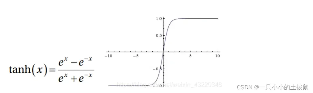
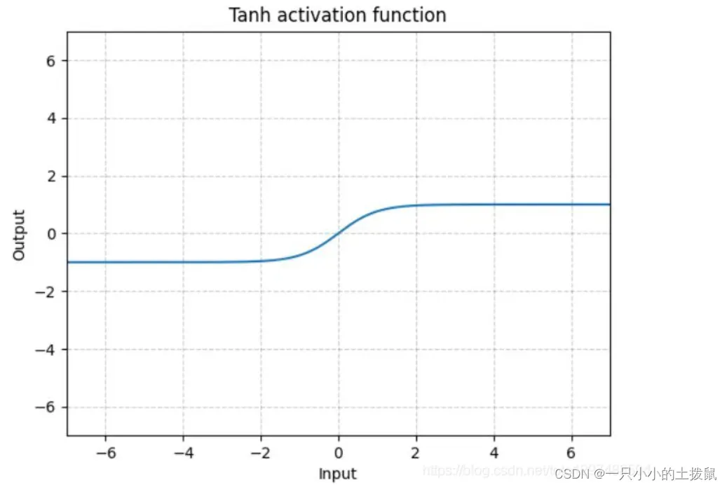 、 Tanh除了居中(-1到1)外,基本上与Sigmoid相同。这个函数的输出的均值大约为0。因此,模型收敛速度更快。注意,如果每个输入变量的平均值接近于0,那么收敛速度通常会更快,原理同Batch Norm。
import torch

x = torch.randn(100, 10)
y = torch.randn(100,30)

func = nn.Tanh()
output_x = func(x)
output_y = func(y)
print("Output size:", output_x.size())
print("Output size:", output_y.size())
# Output size: torch.Size([100, 10])
# Output size: torch.Size([100, 30])
print(x[0])
print(output_x[0])
# tensor([-0.2978, -1.0893, -0.3137, -0.5245, -0.1842,  1.6686, -0.7928, -2.2920, -0.8125, -1.9004])
# tensor([-0.2893, -0.7966, -0.3038, -0.4812, -0.1822,  0.9314, -0.6600, -0.9798,-0.6709, -0.9563])

class Tanh(nn.Module):
	def __init__(self):
		super(Tanh, self).__init__()
	def forward(self, x):
		return (torch.exp(x)-torch.exp(-x))/(torch.exp(x)+torch.exp(-x))

class Tanh(nn.Module):
	def __init__(self):
		super(Tanh, self).__init__()
	def forward(self, x):
		return F.tanh(x)
8、torch.nn.ELU()
数学表达式:
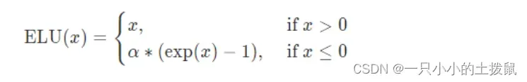
其中α是一个可调整的参数,它控制着ELU负值部分在何时饱和。右侧线性部分使得ELU能够缓解梯度消失,而左侧软饱能够让ELU对输入变化或噪声更鲁棒。ELU的输出均值接近于零,所以收敛速度更快.
ELU不同于ReLU的点是,它可以输出小于0的值,使得系统的平均输出为0。因此,ELU会使得模型收敛的更加快速,其变种(CELU , SELU)只是不同参数组合ELU。
import torch
import torch.nn as nn
x = torch.randn(100, 10)
# torch.nn.SELU(inplace=False)
func = nn.ELU()
y = func(x)
print(x[0])
print(y[0])
# tensor([-0.6763,  0.6669, -2.0544, -1.8889, -0.3581,  0.0884, -1.3734,  0.9181,0.4205,  0.1281])
# tensor([-0.4915,  0.6669, -0.8718, -0.8488, -0.3010,  0.0884, -0.7467,  0.9181,0.4205,  0.1281])


import torch
import torch.nn as nn
import torch.nn.functional as F
import matplotlib.pyplot as plt

class ELU(nn.Module):
    def __init__(self):
        super().__init__()
    def forward(self,x):
        x = F.elu(x)
        return x

class ELU(nn.Module):
    def __init__(self, alpha=1.0):
        super(ELU, self).__init__()
        self.alpha=alpha

    def forward(self, x):
        temp1 = F.relu(x)
        temp2 = self.alpha * (-1*F.relu(1-torch.exp(x)))
        return temp1 + temp2
x = torch.linspace(-10, 10, 1000).unsqueeze(0)

func = nn.ELU()
func2 = ELU()

y1 = func(x)
y2 = func2(x)

plt.plot(x.detach().numpy()[0],y1.detach().numpy()[0],label="PyTorch")
plt.plot(x.detach().numpy()[0],y2.detach().numpy()[0],label="myELU")
plt.legend()
plt.grid()
plt.show()
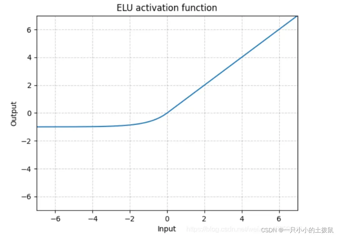
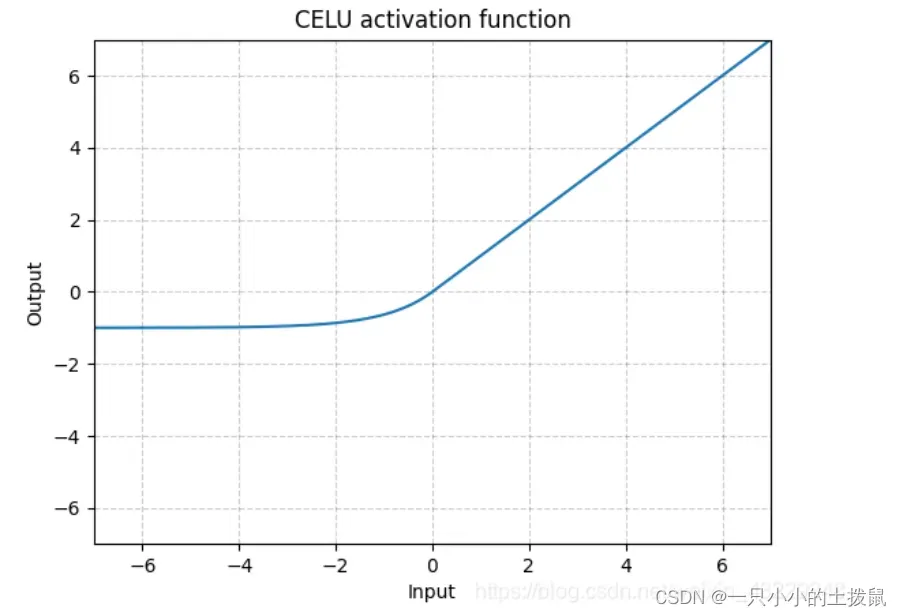
9、torch.nn.CELU()
数学表达式:

跟ELU相比,CELU是将ELU中的exp(x)变为exp(x/a)
import torch
import torch.nn as nn
x = torch.randn(100, 10)
# torch.nn.SELU(inplace=False)
func = nn.CELU()
y = func(x)
print(x[0])
print(y[0])
# tensor([-1.1315, -0.3425,  0.7596, -1.8625, -0.8638,  0.2654,  0.9773, -0.5946, 0.1348, -0.7941])
# tensor([-0.6775, -0.2900,  0.7596, -0.8447, -0.5785,  0.2654,  0.9773, -0.4482, 0.1348, -0.5480])


import torch
import torch.nn as nn
import torch.nn.functional as F
from matplotlib import pyplot as plt
class CELU(nn.Module):
    def __init__(self, alpha=1.0):
        super(CELU, self).__init__()
        self.alpha=alpha

    def forward(self, x):
        temp1 = F.relu(x)
        # temp2 = self.alpha * (F.elu(-1*F.relu(-1.*x/self.alpha)))
        temp2 = self.alpha * (-1*F.relu(1-torch.exp(x/self.alpha)))
        return temp1 + temp2

x = torch.linspace(-10, 10, 1000).unsqueeze(0)

func = nn.CELU()
func2 = CELU()

y1 = func(x)
y2 = func2(x)

plt.plot(x.detach().numpy()[0],y1.detach().numpy()[0],label="PyTorch")
plt.plot(x.detach().numpy()[0],y2.detach().numpy()[0],label="myCELU")
plt.legend()
plt.grid()
plt.show()
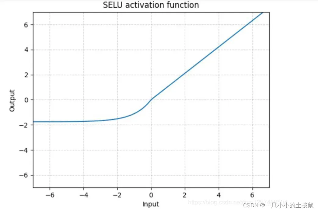
10、torch.nn.SELU()
数学表达式:

此处的scale就是下方的 λ
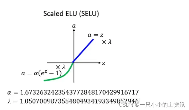
跟ELU相比,SELU是将ELU乘上了一个scala变量。当使用kaiming_normal或kaiming_normal_进行初始化时,为了得到 自归一化 的神经网络,应该使用nonlinearity=’linear’而不是nonlinearity=‘selu’。经过该激活函数后使得样本分布自动归一化到0均值和单位方差(自归一化,保证训练过程中梯度不会爆炸或消失,效果比Batch Normalization 要好)。关键在于这个 λ 是大于1的,在方差过小的的时候可以让它增大,同时防止了梯度消失。
import torch
import torch.nn as nn
import torch.nn.functional as F
from matplotlib import pyplot as plt
class SELU(nn.Module):
    def __init__(self):
        super(SELU, self).__init__()
        self.alpha = 1.6732632423543772848170429916717
        self.scale = 1.0507009873554804934193349852946
    def forward(self, x):
        temp1 = self.scale * F.relu(x)
        # temp2 = self.scale * self.alpha * (F.elu(-1*F.relu(-1*x)))
        temp2 = self.scale * self.alpha * (-1*F.relu(1-torch.exp(x)))
        return temp1 + temp2

x = torch.linspace(-10, 10, 1000).unsqueeze(0)

func2 = nn.SELU()
func = SELU()

y1 = func(x)
y2 = func2(x)

plt.plot(x.detach().numpy()[0],y1.detach().numpy()[0],label="mySELU")
plt.plot(x.detach().numpy()[0],y2.detach().numpy()[0],label="PyTorch")
plt.legend()
plt.grid()
plt.show()
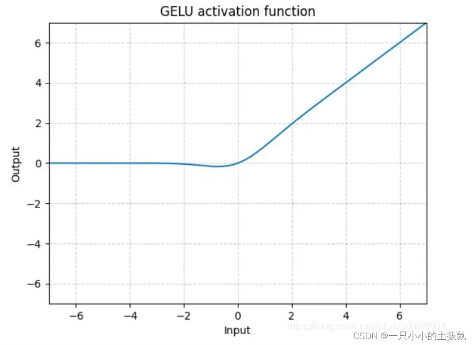
11、torch.nn.GELU()
高斯误差线性单元激活函数在最近的 Transformer 模型中得到了应用。是高斯分布的累积分布函数
数学表达式:

import torch.nn as nn
import torch
import matplotlib.pyplot as plt
import numpy as np

class GELU(nn.Module):
	def __init__(self, beta=1):
		super(GELU, self).__init__()
	def forward(self, x):
		return F.gelu(x)

class GELU(nn.Module):
	def __init__(self, beta=1):
		super(GELU, self).__init__()
	def forward(self, x):
		x_= np.sqrt(2./np.pi) * (x+0.044715 * x * x * x)
		return 0.5 * x * (1 + (torch.exp(x_) - torch.exp(-x_))/(torch.exp(x_) + torch.exp(-x_)))

x = torch.linspace(-10, 10, 1000).unsqueeze(0)
# torch.nn.SELU(inplace=False)
func2 = nn.GELU()
func = GELU()

y1 = func(x)
y2 = func2(x)

plt.plot(x.detach().numpy()[0],y1.detach().numpy()[0],label="myGELU")
plt.plot(x.detach().numpy()[0],y2.detach().numpy()[0],label="PyTorch")
plt.legend()
plt.grid()
plt.show()
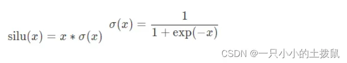
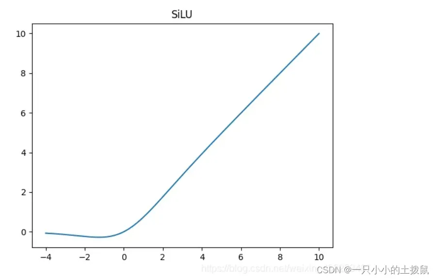
12、torch.nn.SiLU()
数学表达式:
import torch
import torch.nn as nn
import torch.nn.functional as F
from matplotlib import pyplot as plt
class SiLU(nn.Module):
    def __init__(self):
        super(SiLU, self).__init__()
    def forward(self, x):
        return x * F.sigmoid(x)

x = torch.linspace(-10, 10, 1000).unsqueeze(0)
# torch.nn.SELU(inplace=False)
func = nn.SiLU()
func2 = SiLU()

y1 = func(x)
y2 = func2(x)

plt.plot(x.detach().numpy()[0],y1.detach().numpy()[0],label="mySiLU")
plt.plot(x.detach().numpy()[0],y2.detach().numpy()[0],label="PyTorch")
plt.legend()
plt.grid()
plt.show()
13、torch.nn.Softplus()
SoftPlus是一个平滑的近似于ReLU函数,可以用来约束输出总是正的。 Softplus作为损失函数在StyleGAN1和2中都得到了使用,下面分别是其表达式和图解。
数学表达式:
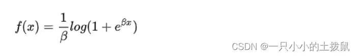
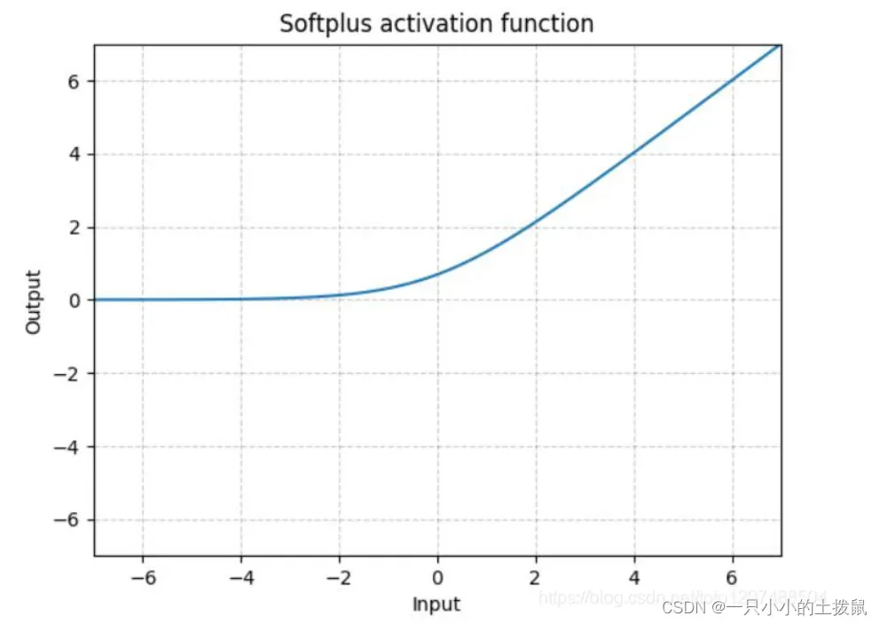
Softplus 是ReLU的光滑近似,可以有效的对输出都为正值的网络进行约束。随着β的增加,Softplus与ReLU越来越接近。
import numpy as np
x = np.linspace(-10, 10, 100)
y1 = np.log(1 + np.exp(x))
y2 = np.maximum(0, x)
plt.plot(x,y1,label="softplus")
plt.plot(x,y2,label="relu")
plt.legend()
plt.show()


import torch
import torch.nn as nn
x = torch.randn(100, 10)
y = torch.randn(100, 30)
# torch.nn.Softplus(beta=1, threshold=20)
func = nn.Softplus()
output_x = func(x)
output_y = func(y)
print("Output size:", output_x.size())
print("Output size:", output_y.size())
# Output size: torch.Size([100, 10])
# Output size: torch.Size([100, 30])
print(x[0])
print(output_x[0])
# tensor([ 2.6387,  0.6161, -0.0684, -0.3626,  2.2955, -0.1481, -0.1116,  0.1727, 0.2522,  0.6943])
# tensor([2.7077, 1.0479, 0.6595, 0.5282, 2.3915, 0.6218, 0.6389, 0.7832, 0.8272, 1.0994])

class Softplus(nn.Module):
	def __init__(self, beta=1):
		super(Softplus, self).__init__()
		self.beta = beta
		assert beta !=0, "beta should not be equal to 0"
	def forward(self, x):
		return 1./beta * torch.log(1 + torch.exp(beta * x))
class Softplus(nn.Module):
	def __init__(self, beta=1.):
		super(Softplus, self).__init__()
		self.beta = beta
		assert beta !=0, "beta should not be equal to 0"
	def forward(self, x):
		return F.softplus(x, beta)
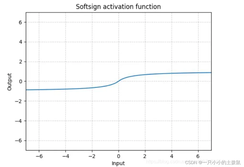
14、torch.nn.Softsign()
同Sigmoid有点类似,但是它比Sigmoid达到渐进线的速度更慢,有效的缓解了梯度消失的问题

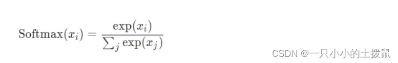
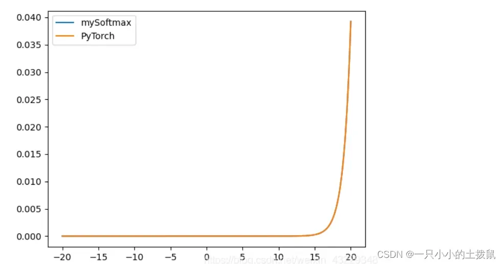
15、torch.nn.Softmax()
Softmax 函数对 n 维输入 Tensor 进行重新缩放,以便 n 维输出 Tensor 的值位于 [0,1] 范围内并且总和为 1。当输入张量是一个稀疏张量时,未指定的值被视为负无穷。
import torch
import torch.nn as nn
import torch.nn.functional as F
from matplotlib import pyplot as plt

class Softmax(nn.Module):
    def __init__(self, dim=1):
        super().__init__()
        self.dim= dim
        print("Softmax activation loaded...")
    def forward(self,X):
    	X_exp = X.exp()
    	partion = X_exp.sum(dim=self.dim, keepdim=True)  # 沿着列方向求和,即对每一行求和
    	return X_exp/partion  # 广播机制,partion被扩展成与X_exp同shape的,对应位置元素做除法

func= Softmax()
x = torch.linspace(-20,20,1000).unsqueeze(0)
y1 = func(x)

func2 = nn.Softmax(dim=1)
y2 = func2(x)

plt.plot(x.detach().numpy()[0],y1.detach().numpy()[0],label="mySoftmax")
plt.plot(x.detach().numpy()[0],y2.detach().numpy()[0],label="PyTorch")
plt.legend()
plt.show()
16、torch.nn.Softmix()
将数字变成概率分布,类似Softmax。
17、torch.nn.Hardtanh()
Hardtanh就是1个线性分段函数[-1, 1],但是用户可以调整下限min_val和上限max_val,使其范围扩大/缩小。

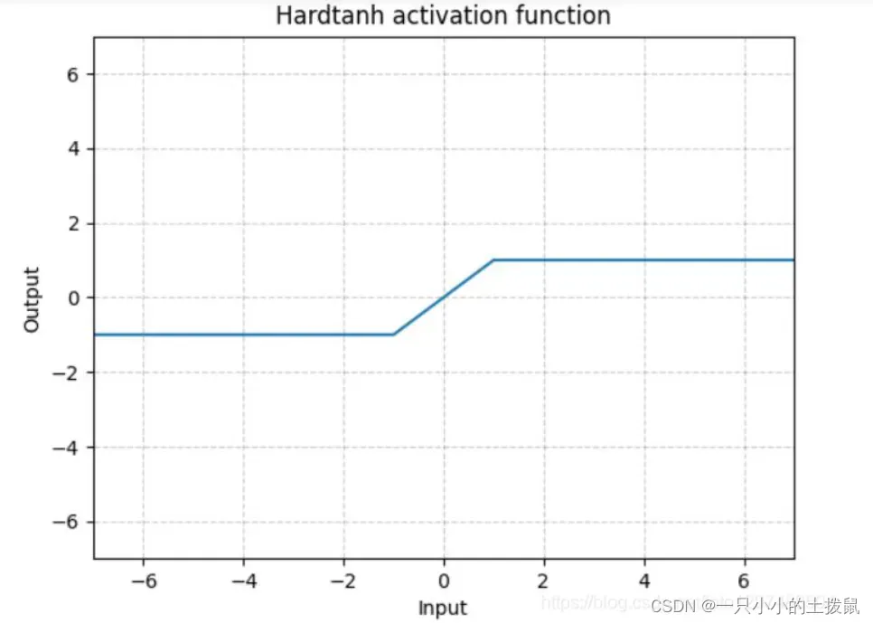
当权值保持在较小的范围内时,Hardtanh的工作效果出奇的好。
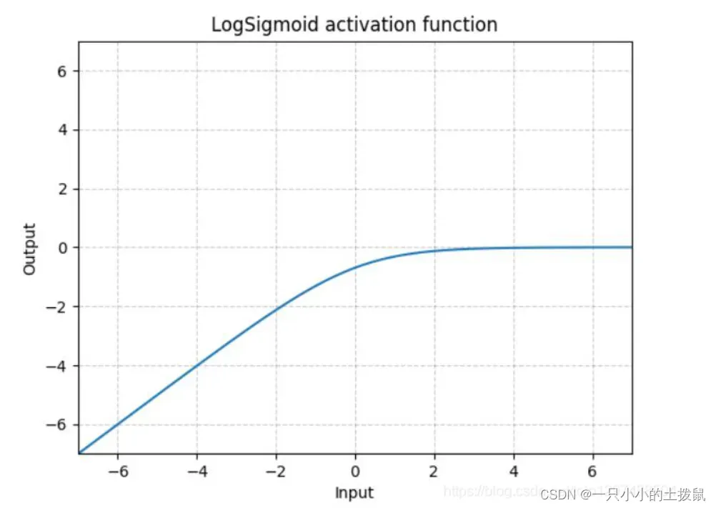
18、torch.nn.LogSigmoid()
下面的公式解释了用于将输入层映射到隐藏层的log sigmoid传递函数。如果数据不是二进制的,并且它是一个浮点类型,有很多异常值(如输入特征中出现的大数值),那么我们应该使用log sigmoid传递函数。 LogSigmoid是在Sigmoid基础上,wrap了一个对数函数。这种方式用作损失函数比较多。

import torch
x = torch.randn(100, 10)
y = torch.randn(100,30)

func = nn.LogSigmoid()
output_x = func(x)
output_y = func(y)
print("Output size:", output_x.size())
print("Output size:", output_y.size())
# Output size: torch.Size([100, 10])
# Output size: torch.Size([100, 30])
print(x[0])
print(output_x[0])
# tensor([-0.6855,  1.1084,  1.0223,  0.8324,  1.0061, -1.4613,  0.7731,  0.0463,0.5831, -0.6826])
# tensor([-1.0935, -0.2852, -0.3073, -0.3612, -0.3116, -1.6699, -0.3795, -0.6702,-0.4435, -1.0916])
19、torch.nn.Softmin()
20、torch.nn.Softmax()
21、torch.nn.LogSoftmax()
参考:
Pytorch的22个激活函数_Wanderer001的博客-CSDN博客_pytorch 激活函数
PyTorch教程(5)激活函数_求则得之,舍则失之的博客-CSDN博客_pytorch 激活函数
Pytorch学习:Task4 PyTorch激活函数原理和使用_奶油松果的博客-CSDN博客
文章出处登录后可见!