泰坦尼克号沉船数据之美——起于悲剧,止于浪漫
前言:泰坦尼克号,不只是卡梅隆导演的经典电影,它是一个真实存在的悲剧,也是电影的故事背景与题材。作为一个IT人,分析事实还得看数据,了解到泰坦尼克号沉船幸存者多为老人、小孩和妇女,而牺牲者多为年轻的男士,这样的历史数据,让我感受到了人性之美与善,七夕,我们一起来分析一下这一悲壮与浪漫的数据吧~
本文内容包含了泰坦尼克号沉船数据分析与可视化、数据建模与分类预测。
现有 titanic.csv 数据集。该数据集记录了泰坦尼克轮船上的乘客信息。使用 scikit-learn 对该数据集进行分析,探究生存率和哪些因素有关(性别,年龄,是否有伴侣,票价,舱位等级,包间,出发地点)。
关键步骤:
1、把数据随机分成训练集和测试集两类。
2、构造特征向量。(注意:如果所选特征是非数值特征,需要将其转成数值。)
3、分别训练判定树、KNN、SVC和朴素贝叶斯四种模型,对测试数据进行预测。
4、使用混淆矩阵对分类器的分类结果进行评估,比较。
5** 绘制ROC曲线。
获取资源:
百度网盘:https://pan.baidu.com/s/1qsY70lqwmgWnMn-A81NOaw
提取码:wsdc
演示环境:Python 3、Jupyter notebook
涉及技术:scikit-learn 分类 + seaborn + matplotlib + pandas +numpy
操作步骤:
导入数据集预处理、特征工程、模型训练和模型对比所需的库
import pandas as pd
import numpy as np
import matplotlib.pyplot as plt
from pylab import *
import seaborn as sns

from sklearn import model_selection, preprocessing, naive_bayes, metrics, svm
from sklearn.model_selection import train_test_split, GridSearchCV
from sklearn.linear_model import LogisticRegression
from sklearn.neighbors import KNeighborsClassifier
from sklearn import ensemble, tree

# 忽略警告提示
import warnings
warnings.filterwarnings('ignore')
1. 数据预处理
1.1 导入数据
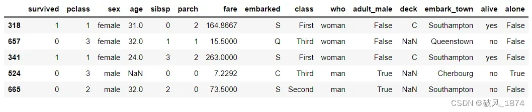
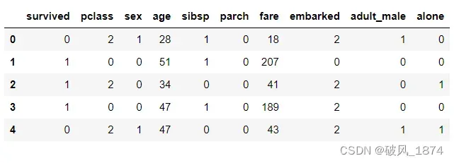
data = pd.read_csv('titanic.csv')
print(data.shape)
data.sample(5)
输出:(891, 15)
1.2 处理缺失值
data.isnull().sum()输出:
survived         0
pclass           0
sex              0
age            177
sibsp            0
parch            0
fare             0
embarked         2
class            0
who              0
adult_male       0
deck           688
embark_town      2
alive            0
alone            0
dtype: int64
缺失值分析:
age、deck、embarked、embark_town 存在缺失值,需要处理。(1)age 对生存率有影响,不能忽略,用平均值填充;(2)总共有 891 条信息,deck 有 688 个缺失值,因此剔除 deck 这个分类标签;(3)embarked、embark_town 缺失值较少,都为 2 个,随机取其中一个数据填充。
data['age']=data['age'].fillna(data['age'].median())
del data['deck']
data['embarked']=data['embarked'].fillna('S')
data['embark_town']=data['embark_town'].fillna('Southampton')

data.isnull().sum()
输出:
survived       0
pclass         0
sex            0
age            0
sibsp          0
parch          0
fare           0
embarked       0
class          0
who            0
adult_male     0
embark_town    0
alive          0
alone          0
dtype: int64
1.3 观察数据
1.3.1 全体成员的生存情况
survived = data['survived'].value_counts().to_frame().reset_index().rename(columns={'index': 'label', 'survived': 'counts'})

#计算存活率
survived_rate = round(342/891, 2)
survived['rate'] = [1-survived_rate, survived_rate]
survived
输出:
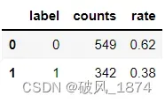
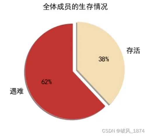
数据描述:存活 的有 342 人,遇难 的有 549 人。
mpl.rcParams['axes.unicode_minus'] = False     #处理无法显示中文的问题
mpl.rcParams['font.sans-serif'] = ['SimHei']

fig=plt.figure(1,figsize=(6,6))
ax1=fig.add_subplot(1,1,1)
label=['遇难','存活']
color=['#C23531','#F5DEB3']
explode=0.05,0.05  #扇区间隔

patches,l_text,p_text = ax1.pie(survived.rate,labels=label,colors=color,startangle=90,autopct='%1.0f%%',explode=explode,shadow=True)
for t in l_text:
    t.set_size(20)
for t in p_text:
    t.set_size(20)
ax1.set_title('全体成员的生存情况', fontsize=20)
输出:
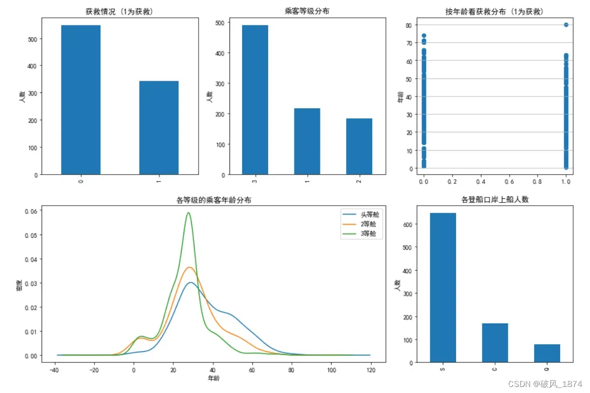
1.3.2 乘客的各属性分布情况
fig = plt.figure(figsize=(15,10))
fig.set(alpha=0.3)  # 设定图表颜色alpha参数(透明度)

plt.subplot2grid((2,3),(0,0))
data.survived.value_counts().plot(kind='bar')
plt.title("获救情况 (1为获救)")
plt.ylabel("人数")

plt.subplot2grid((2,3),(0,1))
data.pclass.value_counts().plot(kind="bar")
plt.ylabel("人数")
plt.title("乘客等级分布")

plt.subplot2grid((2,3),(0,2))
plt.scatter(data.survived, data.age)
plt.ylabel("年龄")
plt.grid(b=True, which='major', axis='y')
plt.title("按年龄看获救分布 (1为获救)")

plt.subplot2grid((2,3),(1,0), colspan=2)
data.age[data.pclass == 1].plot(kind='kde')
data.age[data.pclass == 2].plot(kind='kde')
data.age[data.pclass == 3].plot(kind='kde')
plt.xlabel("年龄")
plt.ylabel("密度")
plt.title("各等级的乘客年龄分布")
plt.legend(('头等舱', '2等舱','3等舱'),loc='best')

plt.subplot2grid((2,3),(1,2))
data.embarked.value_counts().plot(kind='bar')
plt.title("各登船口岸上船人数")
plt.ylabel("人数")
plt.show()
输出:
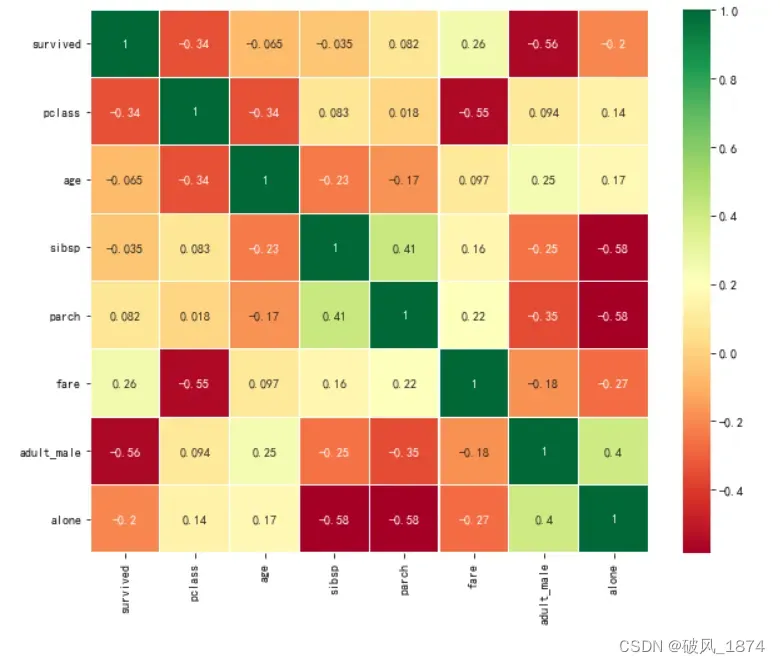
1.3.3 特征之间的相关性
sns.heatmap(data.corr(),annot=True,cmap='RdYlGn',linewidths=0.2)
fig=plt.gcf()
fig.set_size_inches(10,8)
plt.show()
输出:
1.3.4 连续值特征(年龄、船票费用)对生存结果的影响
fig = plt.figure(figsize=(15,4))

plt.subplot2grid((2,2),(0,0))
data.age[data.survived == 0].plot(kind='box', vert=False, patch_artist=True, notch = True, color='#C23531', fontsize=15)
plt.grid(linestyle="--", alpha=0.8)
plt.title("遇难", fontsize=15)

plt.subplot2grid((2,2),(0,1))
data.fare[data.survived == 0].plot(kind='box', vert=False, patch_artist=True, notch = True, color='#C23531', fontsize=15)
plt.grid(linestyle="--", alpha=0.8)
plt.title("遇难", fontsize=15)

plt.subplot2grid((2,2),(1,0))
data.age[data.survived == 1].plot(kind='box', vert=False, patch_artist=True, notch = True, color='#F5DEB3', fontsize=15)
plt.grid(linestyle="--", alpha=0.8)
plt.xlabel("存活", fontsize=15)

plt.subplot2grid((2,2),(1,1))
data.fare[data.survived == 1].plot(kind='box', vert=False, patch_artist=True, notch = True, color='#F5DEB3', fontsize=15)
plt.grid(linestyle="--", alpha=0.8)
plt.xlabel("存活", fontsize=15)
输出: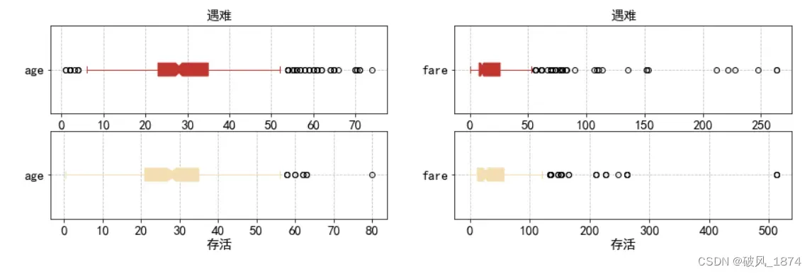
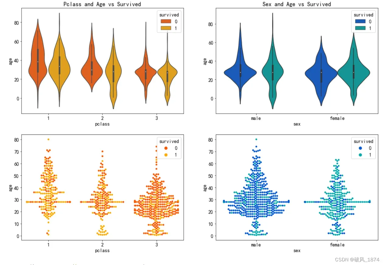
1.3.5 乘客等级、性别对生存结果的影响(从年龄的分布看)
mpl.rcParams.update({'font.size': 14})
fig,axes=plt.subplots(2,2,figsize=(18, 12))
sns.violinplot("pclass","age", hue="survived", data=data, palette='autumn',ax=axes[0][0]).set_title('Pclass and Age vs Survived')
sns.swarmplot(x="pclass", y="age",hue="survived", data=data,palette='autumn',ax=axes[1][0]).legend(loc='upper right').set_title('survived')
sns.violinplot("sex","age", hue="survived", data=data, palette='winter', ax=axes[0][1]).set_title('Sex and Age vs Survived')
sns.swarmplot(x="sex", y="age",hue="survived", data=data,palette='winter',ax=axes[1][1]).legend(loc='upper right').set_title('survived')
输出:
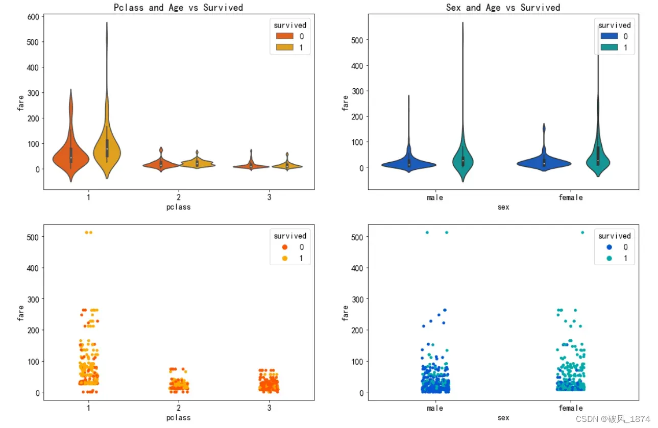
1.3.6 乘客等级、性别对生存结果的影响(从船票费用的分布看)
fig,axes=plt.subplots(2,2,figsize=(18, 12))
sns.violinplot("pclass","fare", hue="survived", data=data, palette='autumn',ax=axes[0][0]).set_title('Pclass and Age vs Survived')
sns.stripplot("pclass", "fare",hue="survived", data=data,palette='autumn',ax=axes[1][0]).legend(loc='upper right').set_title('survived')
sns.violinplot("sex","fare", hue="survived", data=data, palette='winter', ax=axes[0][1]).set_title('Sex and Age vs Survived')
sns.stripplot("sex", "fare",hue="survived", data=data,palette='winter',ax=axes[1][1]).legend(loc='upper right').set_title('survived')
输出:
2. 特征工程
2.1 Feature Preprocessing——标签编码预处理
在所有标签中,survived 是分类标签,其余的 14 个变量是分类特征。 由于特征和标签的值存在非结构化类型,因此需要进行特征工程处理,即进行字符串编码处理。
data.info()输出:
<class 'pandas.core.frame.DataFrame'>
RangeIndex: 891 entries, 0 to 890
Data columns (total 14 columns):
 #   Column       Non-Null Count  Dtype
---  ------       --------------  -----
 0   survived     891 non-null    int64
 1   pclass       891 non-null    int64
 2   sex          891 non-null    object
 3   age          891 non-null    float64
 4   sibsp        891 non-null    int64
 5   parch        891 non-null    int64
 6   fare         891 non-null    float64
 7   embarked     891 non-null    object
 8   class        891 non-null    object
 9   who          891 non-null    object
 10  adult_male   891 non-null    bool
 11  embark_town  891 non-null    object
 12  alive        891 non-null    object
 13  alone        891 non-null    bool
dtypes: bool(2), float64(2), int64(4), object(6)
memory usage: 85.4+ KB
初始化编码器
le = preprocessing.LabelEncoder()
for col in data.columns:
    data[col] = le.fit_transform(data[col])
data.head()
data.to_csv('Preprocessing_Titanic.csv')
2.2 去除多余的的标签
名字对生存率几乎没有影响,所以删除 who 标签
del data['who']去掉意思表达一样的标签
data_ = data.T.drop_duplicates().T
print('去重前:', len(data.columns))
print('去重后:', len(data_.columns))

for a in data.columns:
    if a not in data_.columns:
        for b in data_.columns:
            if list(data[b].values) == list(data[a].values):
                print(f'重复标签: {a} 和 {b}')
data = data_
输出:
去重前: 13
去重后: 10
重复标签: class 和 pclass
重复标签: embark_town 和 embarked
重复标签: alive 和 survived
data.head()输出:
2.3 可视化探索各个特征的分布情况
result_plot = data.hist(bins=50, figsize=(14, 12))输出:
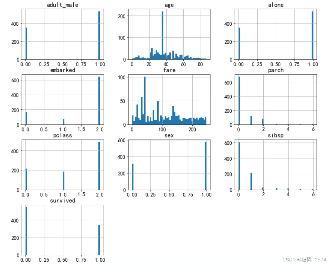
由上面的可视化情况来看,不需要对特征进行标准化处理。
# 对数据进行标准化
# X = StandardScaler().fit_transform(X)
2.4 10折交叉验证分割数据集,9份做训练,1份做测试 ,确保训练和测试数据无交集
X = data.iloc[:, 1:]
y = data.iloc[:, 0]

x_train, x_test, y_train, y_test = train_test_split(X, y,test_size=0.1,shuffle=True,random_state=20)

print(x_train.shape)
print(x_test.shape)
print(y[:5])
X[:5]
输出:
(801, 9)
(90, 9)
0    0
1    1
2    1
3    1
4    0
Name: survived, dtype: int64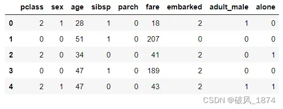
3. 建立模型训练及评估函数
3.1 建模
model, train_score, test_score, roc_auc = [], [], [], []  # 存储相关模型信息,以便后续分析

def train_model(classifier, x_train, y_train, x_test):
    lr = classifier  # 初始化
    lr.fit(x_train, y_train)  # 训练
    y_pred_lr = lr.predict(x_test)  # 预测

    if '.' in str(classifier):
        model_name = str(classifier).split('(')[0].split('Classifier')[0].split('.')[1]
        print('\n{:=^60}'.format(model_name))
    else:
        model_name = str(classifier).split('(')[0].split('Classifier')[0]
        print('\n{:=^60}'.format(model_name))
    model.append(model_name)

    # 性能评估
    print('\n>>>在训练集上的表现:', lr.score(x_train, y_train))
    print('\n>>>在测试集上的表现:', metrics.accuracy_score(y_test, y_pred_lr))
    print('\n>>>预测的 Roc_auc:%.4f' % metrics.roc_auc_score(y_test, y_pred_lr))
    print('\n>>>混淆矩阵'),show_confusion_matrix(metrics.confusion_matrix(y_test,y_pred_lr))

    train_score.append(lr.score(x_train, y_train))
    test_score.append(metrics.accuracy_score(y_test, y_pred_lr))
    roc_auc.append(metrics.roc_auc_score(y_test, y_pred_lr))
3.2 绘制误分类矩阵函数
def show_confusion_matrix(cnf_matrix):
plt.matshow(cnf_matrix,cmap=plt.cm.YlGn,alpha=0.7)
ax=plt.gca()
ax.set_xlabel('Predicted Label',fontsize=16)
ax.set_xticks(range(0,len(survived.label)))
ax.set_xticklabels(survived.label,rotation=45)
ax.set_ylabel('Actual Label',fontsize=16,rotation=90)
ax.set_yticks(range(0,len(survived.label)))
ax.set_yticklabels(survived.label)
ax.xaxis.set_label_position('top')
ax.xaxis.tick_top()
for row in range(len(cnf_matrix)):
for col in range(len(cnf_matrix[row])):
ax.text(col,row,cnf_matrix[row][col],va='center',ha='center',fontsize=16)
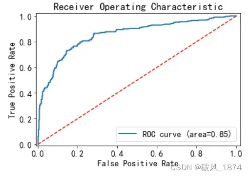
plt.show()3.3 绘制ROC曲线函数
def show_roc_line(classifier, x_train, y_train):
    y_train_prob=classifier.predict_proba(x_train)
    y_pred_prob=y_train_prob[:,1]                             #正例率
    fpr,tpr,thresholds=metrics.roc_curve(y_train,y_pred_prob) #计算ROC曲线
    auc=metrics.auc(fpr,tpr)                                  #计算AUC
    plt.plot(fpr,tpr,lw=2,label='ROC curve (area={:.2f})'.format(auc))
    plt.plot([0,1],[0,1],'r--')
    plt.xlim([-0.01, 1.02])
    plt.ylim([-0.01, 1.02])
    plt.xlabel('False Positive Rate')
    plt.ylabel('True Positive Rate')
    plt.title('Receiver Operating Characteristic')
    plt.legend(loc='lower right')
    plt.show()
4. 训练预测
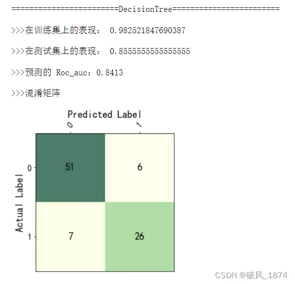
(1) Decision Tree 模型
classifier = tree.DecisionTreeClassifier()
train_model(classifier, x_train, y_train, x_test)  #建模
输出:
可视化特征重要性权重
labels = X.columns
importances = classifier.feature_importances_   # 获取特征权重值
indices = np.argsort(importances)[::-1]# 打印特征等级

features = [labels[i] for i in indices]
weights = [importances[i] for i in indices]

print("Feature ranking:")
for f in range(len(features)):
    print("%d. %s (%f)" % (f + 1, features[f], weights[f]))# 绘制随机森林的特征重要性

plt.figure()
plt.title("Feature importances")
plt.bar(features, np.array(weights), color='r')
plt.xticks(rotation=90)
plt.title('Feature Weights')
plt.show()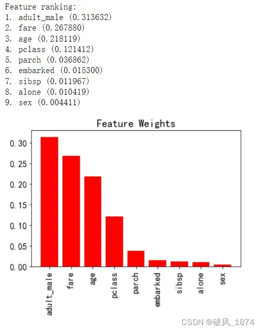
数据分析:从上面的可视化图可以看出,对生存率影响大的特征只有 4 个:fare(船票费用)、adult_male(成年男性)、age(年龄)、pclass(乘客等级)。
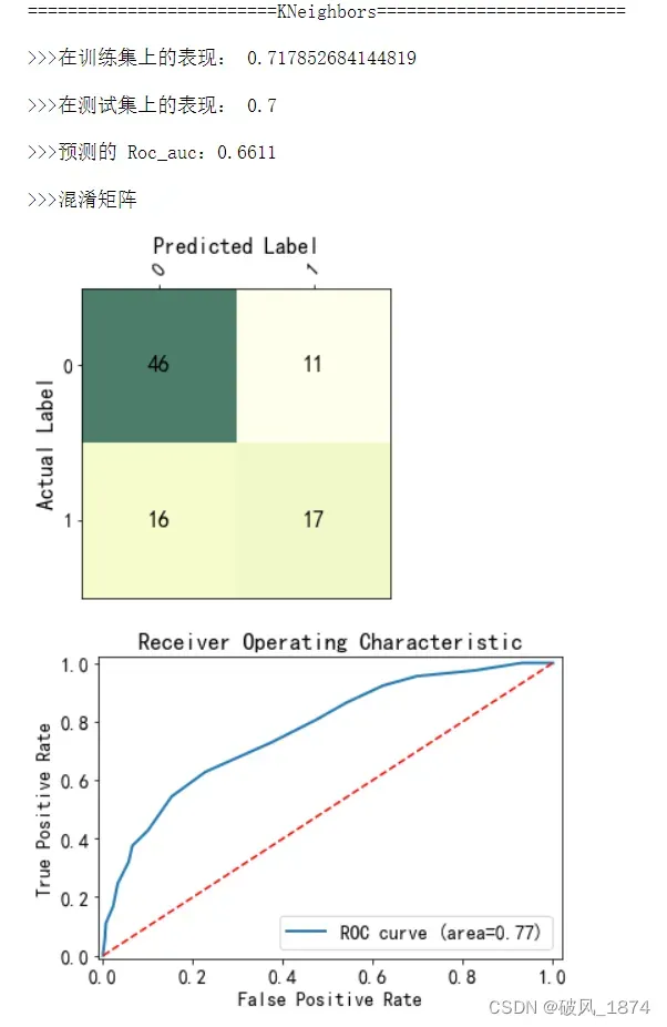
(2) KNN模型
classifier = KNeighborsClassifier(n_neighbors=20)
train_model(classifier, x_train, y_train, x_test)
show_roc_line(classifier, x_train, y_train)
输出:
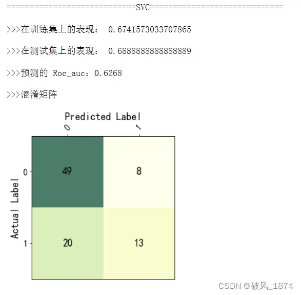
(3) SVC模型
classifier = svm.SVC()
train_model(classifier, x_train, y_train, x_test)
输出:
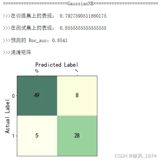
(4) 朴素贝叶斯
classifier = naive_bayes.GaussianNB()
train_model(classifier, x_train, y_train, x_test)  #建模
输出:
show_roc_line(classifier, x_train, y_train) #绘制ROC曲线输出:
5. 性能比较
比较不同模型之间的性能情况
df = pd.DataFrame()
df['model'] = model
df['Roc_auc'] = roc_auc
df['train_score'] = train_score
df['test_score'] = test_score
df
输出:
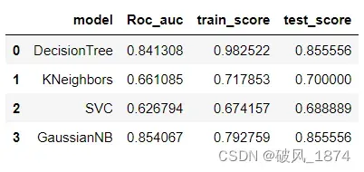
【评判标准:AUC(Area under Curve),Roc曲线下的面积,介于0.1和1之间。Auc作为数值可以直观的评价分类器的好坏,值越大越好。】
从上面的结果可以看出,朴素贝叶斯(GaussianNB)的 Roc_auc 分值最高,预测结果最好,说明朴素贝叶斯比较适合泰坦尼克号问题的分类。
特别的,对于 DecisionTree 的训练和预测结果,可以看出训练集拟合非常好,但是测试集拟合较差,说明过拟合了,需要调参:
param = [{'criterion':['gini'],'max_depth': np.arange(20,50,10),'min_samples_leaf':np.arange(2,8,2),
          'min_impurity_decrease':np.linspace(0.1,0.9,10)},
         {'criterion':['gini','entropy']},
         {'min_impurity_decrease':np.linspace(0.1,0.9,10)}]
clf = GridSearchCV(tree.DecisionTreeClassifier(),param_grid=param,cv=10)
clf.fit(x_train,y_train)
print('最优参数:', clf.best_params_)
print('最好成绩:', clf.best_score_)
输出:
最优参数: {'criterion': 'gini', 'max_depth': 20, 'min_impurity_decrease': 0.1, 'min_samples_leaf': 2}
最好成绩: 0.7839814814814815
按最优参数生成决策树
model = tree.DecisionTreeClassifier(criterion= 'gini', max_depth=20, min_impurity_decrease=0.1, min_samples_leaf= 2)
model.fit(x_train, y_train)
y_pred = model.predict(x_test)
print('train score:', clf.score(x_train, y_train))
print('test score:', clf.score(x_test, y_test))
print("查准率:", metrics.precision_score(y_test,y_pred))
print('召回率:',metrics.recall_score(y_test,y_pred))
print('f1分数:', metrics.f1_score(y_test,y_pred)) #二分类评价标准
输出:
train score: 0.784019975031211
test score: 0.8333333333333334
查准率: 0.7647058823529411
召回率: 0.7878787878787878
f1分数: 0.7761194029850745
从上面的分值来看,按最优参数生成决策树的预测结果比较理想,但还是比朴素贝叶斯(GaussianNB)的预测分值差一些,比其他模型的预测分值好。
【最后,祝大家七夕快乐,顺便记得给我点个赞~~~~】
【同时,欢迎留言、讨论~~~】
文章出处登录后可见!