欢迎关注笔者的微信公众号

Proplot

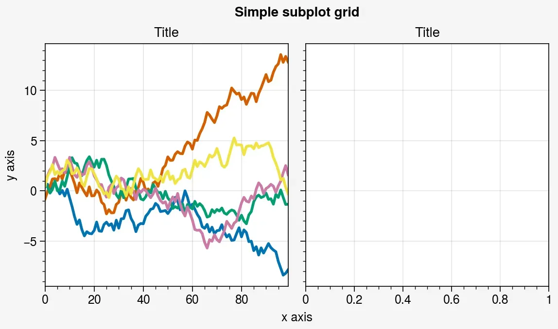
要使用proplot绘图，必须先调用 figure 或 subplots 。这些是根据同名的 pyplot 命令建模的。跟matplotlib.pyplot 一样，subplots 一次创建一个图形和一个子图网格，而 figure 创建一个空图形，之后可以用子图填充。下面显示了一个只有一个子图的最小示例。

安装

pip install proplot
conda install -c conda-forge proplot

# Simple subplot grid
import numpy as np
import proplot as pplt
import warnings
warnings.filterwarnings('ignore')
state = np.random.RandomState(51423)
data = 2 * (state.rand(100, 5) - 0.5).cumsum(axis=0)
fig = pplt.figure()
ax = fig.subplot(121)
ax.plot(data, lw=2)
ax = fig.subplot(122)
fig.format(
    suptitle='Simple subplot grid', title='Title',
    xlabel='x axis', ylabel='y axis'
)
# fig.save('~/example1.png')  # save the figure
# fig.savefig('~/example1.png')  # alternative

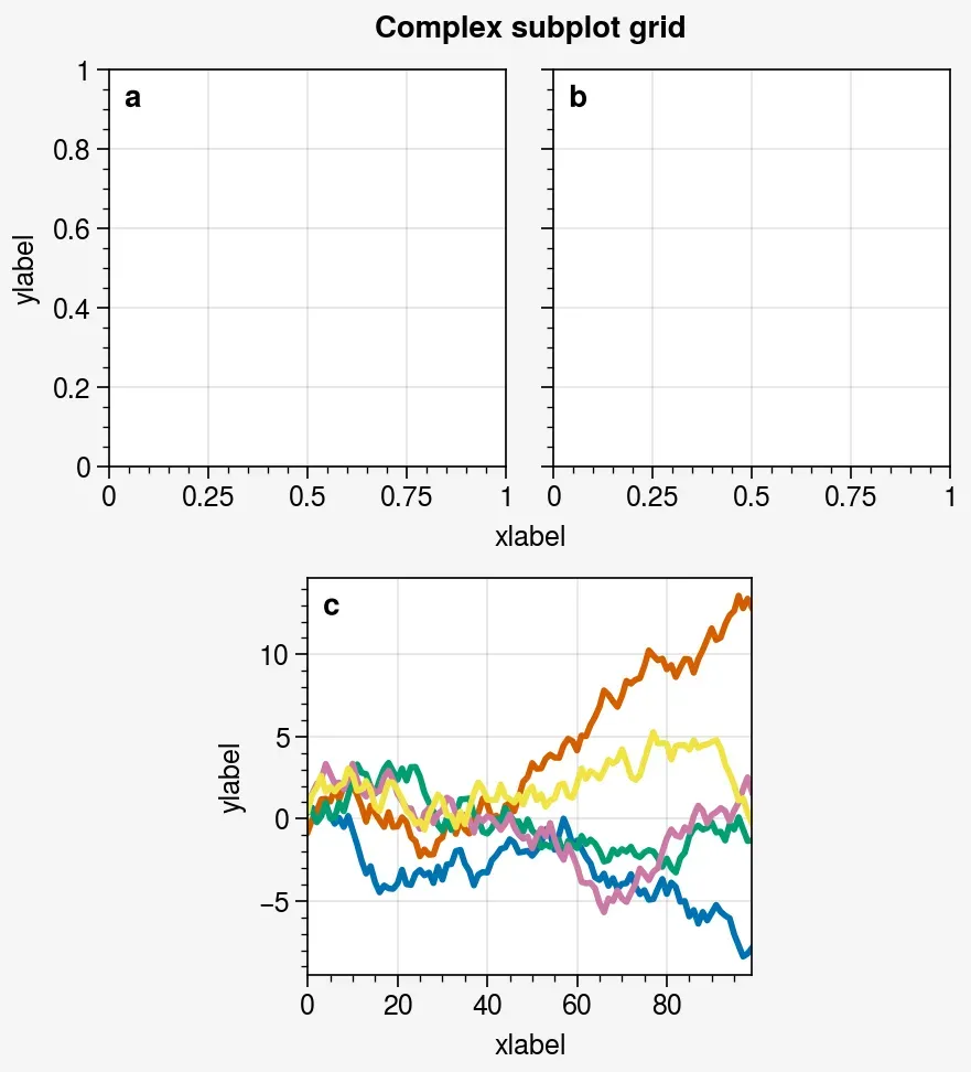
# Complex grid
import numpy as np
import proplot as pplt
state = np.random.RandomState(51423)
data = 2 * (state.rand(100, 5) - 0.5).cumsum(axis=0)
array = [  # the "picture" (0 == nothing, 1 == subplot A, 2 == subplot B, etc.)
    [1, 1, 2, 2],
    [0, 3, 3, 0],
]
fig = pplt.figure(refwidth=1.8)
axs = fig.subplots(array)
axs.format(
    abc=True, abcloc='ul', suptitle='Complex subplot grid',
    xlabel='xlabel', ylabel='ylabel'
)
axs[2].plot(data, lw=2)
# fig.save('~/example2.png')  # save the figure
# fig.savefig('~/example2.png')  # alternative

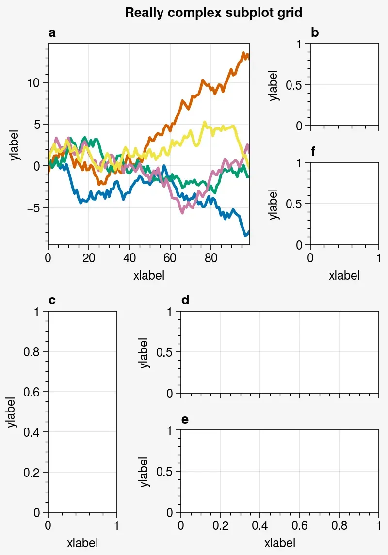
# Really complex grid
import numpy as np
import proplot as pplt
state = np.random.RandomState(51423)
data = 2 * (state.rand(100, 5) - 0.5).cumsum(axis=0)
array = [  # the "picture" (1 == subplot A, 2 == subplot B, etc.)
    [1, 1, 2],
    [1, 1, 6],
    [3, 4, 4],
    [3, 5, 5],
]
fig, axs = pplt.subplots(array, figwidth=5, span=False)
axs.format(
    suptitle='Really complex subplot grid',
    xlabel='xlabel', ylabel='ylabel', abc=True
)
axs[0].plot(data, lw=2)
# fig.save('~/example3.png')  # save the figure
# fig.savefig('~/example3.png')  # alternative

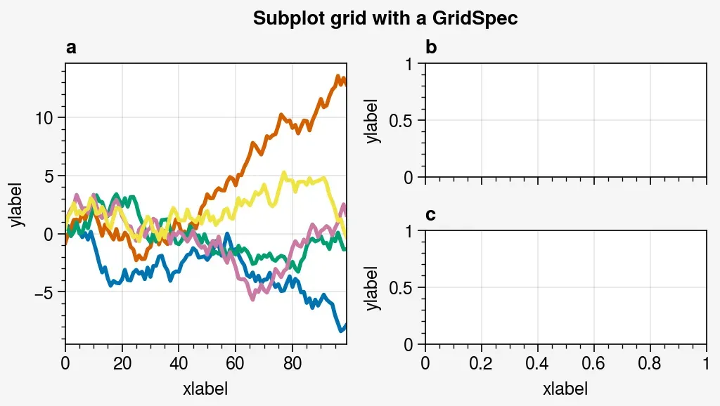
# Using a GridSpec
import numpy as np
import proplot as pplt
state = np.random.RandomState(51423)
data = 2 * (state.rand(100, 5) - 0.5).cumsum(axis=0)
gs = pplt.GridSpec(nrows=2, ncols=2, pad=1)
fig = pplt.figure(span=False, refwidth=2)
ax = fig.subplot(gs[:, 0])
ax.plot(data, lw=2)
ax = fig.subplot(gs[0, 1])
ax = fig.subplot(gs[1, 1])
fig.format(
    suptitle='Subplot grid with a GridSpec',
    xlabel='xlabel', ylabel='ylabel', abc=True
)
# fig.save('~/example4.png')  # save the figure
# fig.savefig('~/example4.png')  # alternative

​
​

import proplot as pplt
import numpy as np
state = np.random.RandomState(51423)

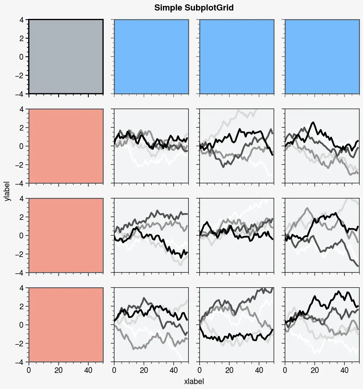
# Selected subplots in a simple grid
fig, axs = pplt.subplots(ncols=4, nrows=4, refwidth=1.2, span=True)
axs.format(xlabel='xlabel', ylabel='ylabel', suptitle='Simple SubplotGrid')
axs.format(grid=False, xlim=(0, 50), ylim=(-4, 4))
axs[:, 0].format(facecolor='blush', edgecolor='gray7', linewidth=1)  # eauivalent
axs[:, 0].format(fc='blush', ec='gray7', lw=1)
axs[0, :].format(fc='sky blue', ec='gray7', lw=1)
axs[0].format(ec='black', fc='gray5', lw=1.4)
axs[1:, 1:].format(fc='gray1')
for ax in axs[1:, 1:]:
    ax.plot((state.rand(50, 5) - 0.5).cumsum(axis=0), cycle='Grays', lw=2)

# Selected subplots in a complex grid
fig = pplt.figure(refwidth=1, refnum=5, span=False)
axs = fig.subplots([[1, 1, 2], [3, 4, 2], [3, 4, 5]], hratios=[2.2, 1, 1])
axs.format(xlabel='xlabel', ylabel='ylabel', suptitle='Complex SubplotGrid')
axs[0].format(ec='black', fc='gray1', lw=1.4)
axs[1, 1:].format(fc='blush')
axs[1, :1].format(fc='sky blue')
axs[-1, -1].format(fc='gray4', grid=False)
axs[0].plot((state.rand(50, 10) - 0.5).cumsum(axis=0), cycle='Grays_r', lw=2)