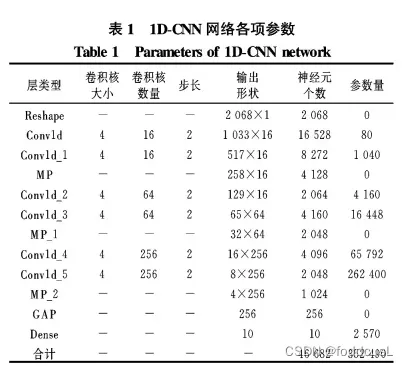
1DCNN 简介:
1D-CNN(一维卷积神经网络)是一种特殊类型的卷积神经网络,设计用于处理一维序列数据。这种网络结构通常由多个卷积层和池化层交替组成,最后使用全连接层将提取的特征映射到输出。
以下是1D-CNN的主要组成部分和特点:
- 输入层:接收一维序列数据作为模型的输入。
- 卷积层:使用一系列可训练的卷积核在输入数据上滑动并提取特征。卷积操作能够有效地提取局部信息,从而捕捉输入序列的局部模式。
- 激活函数:对卷积层的输出进行非线性变换,增强模型的表达能力。
- 池化层:通过对卷积层输出进行降维,减少计算量,同时提高模型的鲁棒性和泛化能力。
- 全连接层:将池化层的输出映射到模型的输出,通常用于分类、回归等任务。
在使用1D-CNN时,通常需要设置一些超参数,如卷积核的大小、卷积层的个数、池化操作的方式、激活函数的选择等。
与传统机器学习对比:
首先,1D-CNN是一种深度学习模型,它使用卷积层来自动提取一维序列数据(如音频、文本等)中的特征。这种方式与传统机器学习中的特征提取方法不同,传统机器学习通常需要手动设计和选择特征。通过自动提取特征,1D-CNN能够减少人工特征提取的工作量,并有可能发现更复杂的特征表示。其次,1D-CNN在处理序列数据时能够更好地捕捉局部关系。卷积操作通过在输入数据上滑动固定大小的窗口来提取局部特征,这使得1D-CNN在语音识别、自然语言处理、时间序列预测等任务中表现出色。而传统机器学习模型,如支持向量机(SVM)或决策树,通常不具备这种处理局部关系的能力。
需要注意的是,在数据尺度较小的时候,如只有100多个参数,相较于传统机器学习模型,1D-CNN并没有优势,表现性能一般和机器学习表现无明显差距。鉴于卷积对于目标特征的提取及压缩的特点,数据长度(参数)越高,1D-CNN就越发有优势。因此在时序回归、高光谱分析、股票预测、音频分析上1D-CNN的表现可圈可点。此外,利用1D-CNN做回归和分类对样本量有较高的要求,因为卷积结构本身对噪声就比较敏感,数据集较少时,特别容易发生严重的过拟合现象,建议样本量800+有比较好的应用效果。
三种不同结构的自定义的1D-CNN
基于VGG结构的1D-CNN(VNet)
基于 VGG 主干网 络设计的 VNet 参考了陈庆等的优化结构,卷积核大 小为 4,包含 6 个卷积深度,并在每个平均池化层后引 入一个比例为 0.3 的随机失活层(dropout layer)防止过拟合,参数量为342K。
matlab构建代码:
function layers=creatCNN2D_VGG(inputsize)
filter=16;
layers = [
    imageInputLayer([inputsize],"Name","imageinput")
    convolution2dLayer([1 4],filter,"Name","conv","Padding","same")
    convolution2dLayer([1 4],filter,"Name","conv_1","Padding","same")
    maxPooling2dLayer([1 2],"Name","maxpool","Padding","same","Stride",[1 2])
    convolution2dLayer([1 4],filter*2,"Name","conv_2","Padding","same")
    convolution2dLayer([1 4],filter*2,"Name","conv_3","Padding","same")
    maxPooling2dLayer([1 2],"Name","maxpool_1","Padding","same","Stride",[1 2])
    fullyConnectedLayer(filter*8,"Name","fc")
    fullyConnectedLayer(1,"Name","fc_1")
    regressionLayer("Name","regressionoutput")];
基于EfficienNet结构的1D-CNN (ENet)
ENet 采用 Swish 激活函数,引入了跳跃连接与 SE(squeeze and excitation)注意力机制,其不仅能有效 实现更深的卷积深度,还能对通道方向上的数据特征进 行感知,在数据尺度较大时,有一定优势。参数量170.4K
生成代码:
function lgraph=creatCNN2D_EffiPlus2(inputsize)

filter=8;
lgraph = layerGraph();

tempLayers = [
    imageInputLayer([1 1293 1],"Name","imageinput")
    convolution2dLayer([1 3],filter,"Name","conv_11","Padding","same","Stride",[1 2])%'DilationFactor',[1,2]
    batchNormalizationLayer("Name","batchnorm_8")
    swishLayer("Name","swish_1_1_1")];
lgraph = addLayers(lgraph,tempLayers);

tempLayers = [
    convolution2dLayer([1 3],filter,"Name","conv_1_1","Padding","same","Stride",[1 1])%%
    batchNormalizationLayer("Name","batchnorm_1_1")
    swishLayer("Name","swish_1_5")];
lgraph = addLayers(lgraph,tempLayers);

tempLayers = [
    globalAveragePooling2dLayer("Name","gapool_1_1")
    convolution2dLayer([1 1],2,"Name","conv_2_1_1","Padding","same")
    swishLayer("Name","swish_2_1_1")
    convolution2dLayer([1 1],filter,"Name","conv_3_1_1","Padding","same")
    sigmoidLayer("Name","sigmoid_1_1")];
lgraph = addLayers(lgraph,tempLayers);

tempLayers = [
    multiplicationLayer(2,"Name","multiplication_3")
    convolution2dLayer([1 3],filter*2,"Name","conv","Padding","same","Stride",[1 2])
    batchNormalizationLayer("Name","batchnorm")
    swishLayer("Name","swish_1_1")];
lgraph = addLayers(lgraph,tempLayers);

tempLayers = [
    convolution2dLayer([1 3],filter*2,"Name","conv_1","Padding","same","Stride",[1 1])%%
    batchNormalizationLayer("Name","batchnorm_1")
    swishLayer("Name","swish_1")];
lgraph = addLayers(lgraph,tempLayers);

tempLayers = [
    globalAveragePooling2dLayer("Name","gapool_1")
    convolution2dLayer([1 1],4,"Name","conv_2_1","Padding","same")
    swishLayer("Name","swish_2_1")
    convolution2dLayer([1 1],filter*2,"Name","conv_3_1","Padding","same")
    sigmoidLayer("Name","sigmoid_1")];
lgraph = addLayers(lgraph,tempLayers);

tempLayers = [
    multiplicationLayer(2,"Name","multiplication")
    convolution2dLayer([1 3],filter*4,"Name","conv_9","Padding","same","Stride",[1 2])
    batchNormalizationLayer("Name","batchnorm_6")
    swishLayer("Name","swish_1_4")];
lgraph = addLayers(lgraph,tempLayers);

tempLayers = [
    convolution2dLayer([1 3],filter*4,"Name","conv_10","Padding","same","Stride",[1 1])%%
    batchNormalizationLayer("Name","batchnorm_7")
    swishLayer("Name","swish_1_3")];
lgraph = addLayers(lgraph,tempLayers);

tempLayers = [
    globalAveragePooling2dLayer("Name","gapool_2")
    convolution2dLayer([1 1],8,"Name","conv_2_2","Padding","same")
    swishLayer("Name","swish_2_2")
    convolution2dLayer([1 1],filter*4,"Name","conv_3_2","Padding","same")
    sigmoidLayer("Name","sigmoid_2")];
lgraph = addLayers(lgraph,tempLayers);

tempLayers = [
    multiplicationLayer(2,"Name","multiplication_2")
    convolution2dLayer([1 3],filter*8,"Name","conv_5","Padding","same","Stride",[1 2])
    batchNormalizationLayer("Name","batchnorm_2")];
lgraph = addLayers(lgraph,tempLayers);

tempLayers = [
    convolution2dLayer([1 1],filter*8,"Name","conv_6","Padding","same")
    batchNormalizationLayer("Name","batchnorm_3")
    swishLayer("Name","swish")
    convolution2dLayer([1 3],filter*8,"Name","conv_7","Padding","same")
    batchNormalizationLayer("Name","batchnorm_4")
    swishLayer("Name","swish_1_2")];
lgraph = addLayers(lgraph,tempLayers);

tempLayers = [
    globalAveragePooling2dLayer("Name","gapool")
    convolution2dLayer([1 1],12,"Name","conv_2","Padding","same")
    swishLayer("Name","swish_2")
    convolution2dLayer([1 1],filter*8,"Name","conv_3","Padding","same")
    sigmoidLayer("Name","sigmoid")];
lgraph = addLayers(lgraph,tempLayers);

tempLayers = [
    multiplicationLayer(2,"Name","multiplication_1")
    convolution2dLayer([1 3],filter*8,"Name","conv_8","Padding","same")
    batchNormalizationLayer("Name","batchnorm_5")];
lgraph = addLayers(lgraph,tempLayers);

tempLayers = [
    additionLayer(2,"Name","addition")
    convolution2dLayer([1 3],1,"Name","conv_4","Padding","same")
    swishLayer("Name","swish_3")
    averagePooling2dLayer([1 3],"Name","avgpool2d","Padding","same")
    fullyConnectedLayer(1,"Name","fc")
    regressionLayer("Name","regressionoutput")];
lgraph = addLayers(lgraph,tempLayers);

lgraph = connectLayers(lgraph,"swish_1_1_1","conv_1_1");
lgraph = connectLayers(lgraph,"swish_1_1_1","gapool_1_1");
lgraph = connectLayers(lgraph,"swish_1_5","multiplication_3/in1");
lgraph = connectLayers(lgraph,"sigmoid_1_1","multiplication_3/in2");
lgraph = connectLayers(lgraph,"swish_1_1","conv_1");
lgraph = connectLayers(lgraph,"swish_1_1","gapool_1");
lgraph = connectLayers(lgraph,"swish_1","multiplication/in1");
lgraph = connectLayers(lgraph,"sigmoid_1","multiplication/in2");
lgraph = connectLayers(lgraph,"swish_1_4","conv_10");
lgraph = connectLayers(lgraph,"swish_1_4","gapool_2");
lgraph = connectLayers(lgraph,"swish_1_3","multiplication_2/in1");
lgraph = connectLayers(lgraph,"sigmoid_2","multiplication_2/in2");
lgraph = connectLayers(lgraph,"batchnorm_2","conv_6");
lgraph = connectLayers(lgraph,"batchnorm_2","addition/in2");
lgraph = connectLayers(lgraph,"swish_1_2","gapool");
lgraph = connectLayers(lgraph,"swish_1_2","multiplication_1/in1");
lgraph = connectLayers(lgraph,"sigmoid","multiplication_1/in2");
lgraph = connectLayers(lgraph,"batchnorm_5","addition/in1");
基于ResNet结构的1D-CNN (RNet)
RNet 由 3 层残差网络模块构成,其结构相较 于 ENet 较为精简,模型容量更少,个人感觉性能比较综合。参数量33.7K
function lgraph=creatCNN2D_ResNet(inputsize)
lgraph = layerGraph();
filter=16;

tempLayers = [
    imageInputLayer([inputsize],"Name","imageinput")
    convolution2dLayer([1 3],filter,"Name","conv","Padding","same","Stride",[1 2])
    batchNormalizationLayer("Name","batchnorm")
    reluLayer("Name","relu")
    maxPooling2dLayer([1 3],"Name","maxpool","Padding",'same',"Stride",[1 2])];
lgraph = addLayers(lgraph,tempLayers);

tempLayers = [
    convolution2dLayer([1 3],filter,"Name","conv_1","Padding","same")
    batchNormalizationLayer("Name","batchnorm_1")
    reluLayer("Name","relu_1")
    convolution2dLayer([1 3],filter,"Name","conv_2","Padding","same")
    batchNormalizationLayer("Name","batchnorm_2")];
lgraph = addLayers(lgraph,tempLayers);

tempLayers = [
    additionLayer(2,"Name","addition")
    reluLayer("Name","relu_3")];
lgraph = addLayers(lgraph,tempLayers);

tempLayers = [
    convolution2dLayer([1 3],filter*2,"Name","conv_3","Padding","same","Stride",[1 2])
    batchNormalizationLayer("Name","batchnorm_3")
    reluLayer("Name","relu_2")
    convolution2dLayer([1 3],filter*2,"Name","conv_4","Padding","same")
    batchNormalizationLayer("Name","batchnorm_4")];
lgraph = addLayers(lgraph,tempLayers);

tempLayers = [
    convolution2dLayer([1 3],filter*2,"Name","conv_8","Padding","same","Stride",[1 2])
    batchNormalizationLayer("Name","batchnorm_8")];
lgraph = addLayers(lgraph,tempLayers);

tempLayers = [
    additionLayer(2,"Name","addition_1")
    reluLayer("Name","relu_5")];
lgraph = addLayers(lgraph,tempLayers);

tempLayers = [
    convolution2dLayer([1 3],filter*4,"Name","conv_5","Padding","same","Stride",[1 2])
    batchNormalizationLayer("Name","batchnorm_5")
    reluLayer("Name","relu_4")
    convolution2dLayer([1 3],filter*4,"Name","conv_6","Padding","same")
    batchNormalizationLayer("Name","batchnorm_6")];
lgraph = addLayers(lgraph,tempLayers);

tempLayers = [
    convolution2dLayer([1 3],filter*4,"Name","conv_7","Padding","same","Stride",[1 2])
    batchNormalizationLayer("Name","batchnorm_7")];
lgraph = addLayers(lgraph,tempLayers);

tempLayers = [
    additionLayer(2,"Name","addition_2")
    reluLayer("Name","res3a_relu")
    globalMaxPooling2dLayer("Name","gmpool")
    fullyConnectedLayer(1,"Name","fc")
    regressionLayer("Name","regressionoutput")];
lgraph = addLayers(lgraph,tempLayers);


lgraph = connectLayers(lgraph,"maxpool","conv_1");
lgraph = connectLayers(lgraph,"maxpool","addition/in2");
lgraph = connectLayers(lgraph,"batchnorm_2","addition/in1");
lgraph = connectLayers(lgraph,"relu_3","conv_3");
lgraph = connectLayers(lgraph,"relu_3","conv_8");
lgraph = connectLayers(lgraph,"batchnorm_4","addition_1/in1");
lgraph = connectLayers(lgraph,"batchnorm_8","addition_1/in2");
lgraph = connectLayers(lgraph,"relu_5","conv_5");
lgraph = connectLayers(lgraph,"relu_5","conv_7");
lgraph = connectLayers(lgraph,"batchnorm_6","addition_2/in1");
lgraph = connectLayers(lgraph,"batchnorm_7","addition_2/in2");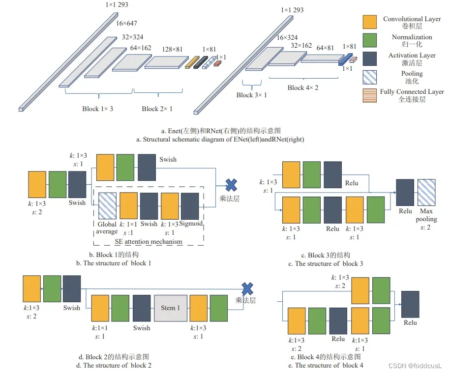
ENet和RNet的结构示意图
训练代码与案例:
训练代码
我们基于RNet采用1293长度的数据对样本进行训练,做回归任务,代码如下:
clear all

load("TestData2.mat");

%数据分割
%[AT,AP]=ks(Alltrain,588);
num_div=1;

%直接载入数据


[numsample,sampleSize]=size(AT);
for i=1:numsample
    XTrain(:,:,1,i)=AT(i,1:end-num_div);
    YTrain(i,1)=AT(i,end);
end
[numtest,~]=size(AP)
for i=1:numtest
    XTest(:,:,1,i)=AP(i,1:end-num_div);
    YTest(i,1)=AP(i,end);
end


%Ytrain=inputData(:,end);
figure
histogram(YTrain)
axis tight
ylabel('Counts')
xlabel('TDS')

options = trainingOptions('adam', ...
    'MaxEpochs',150, ...
    'MiniBatchSize',64, ...
    'InitialLearnRate',0.008, ...
    'GradientThreshold',1, ...
    'Verbose',false,...
    'Plots','training-progress',...
    'ValidationData',{XTest,YTest});

layerN=creatCNN2D_ResNet([1,1293,1]);%创建网络,根据自己的需求改函数名称

[Net, traininfo] = trainNetwork(XTrain,YTrain,layerN,options);


YPredicted = predict(Net,XTest);
predictionError = YTest- YPredicted;
squares = predictionError.^2;
rmse = sqrt(mean(squares))
[R P] = corrcoef(YTest,YPredicted)
scatter(YPredicted,YTest,'+')
xlabel("Predicted Value")
ylabel("True Value")
R2=R(1,2)^2;
hold on
plot([0 2000], [-0 2000],'r--')
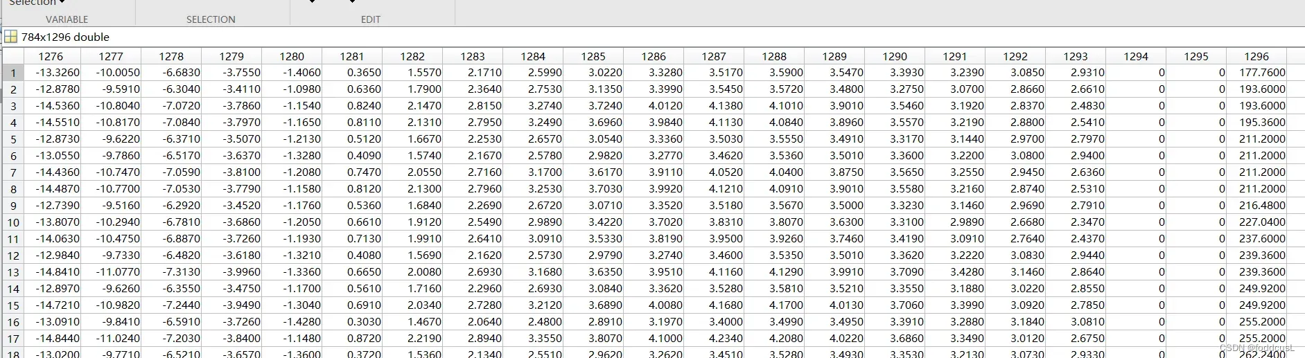
训练数据输入如下:最后一列为预测值:
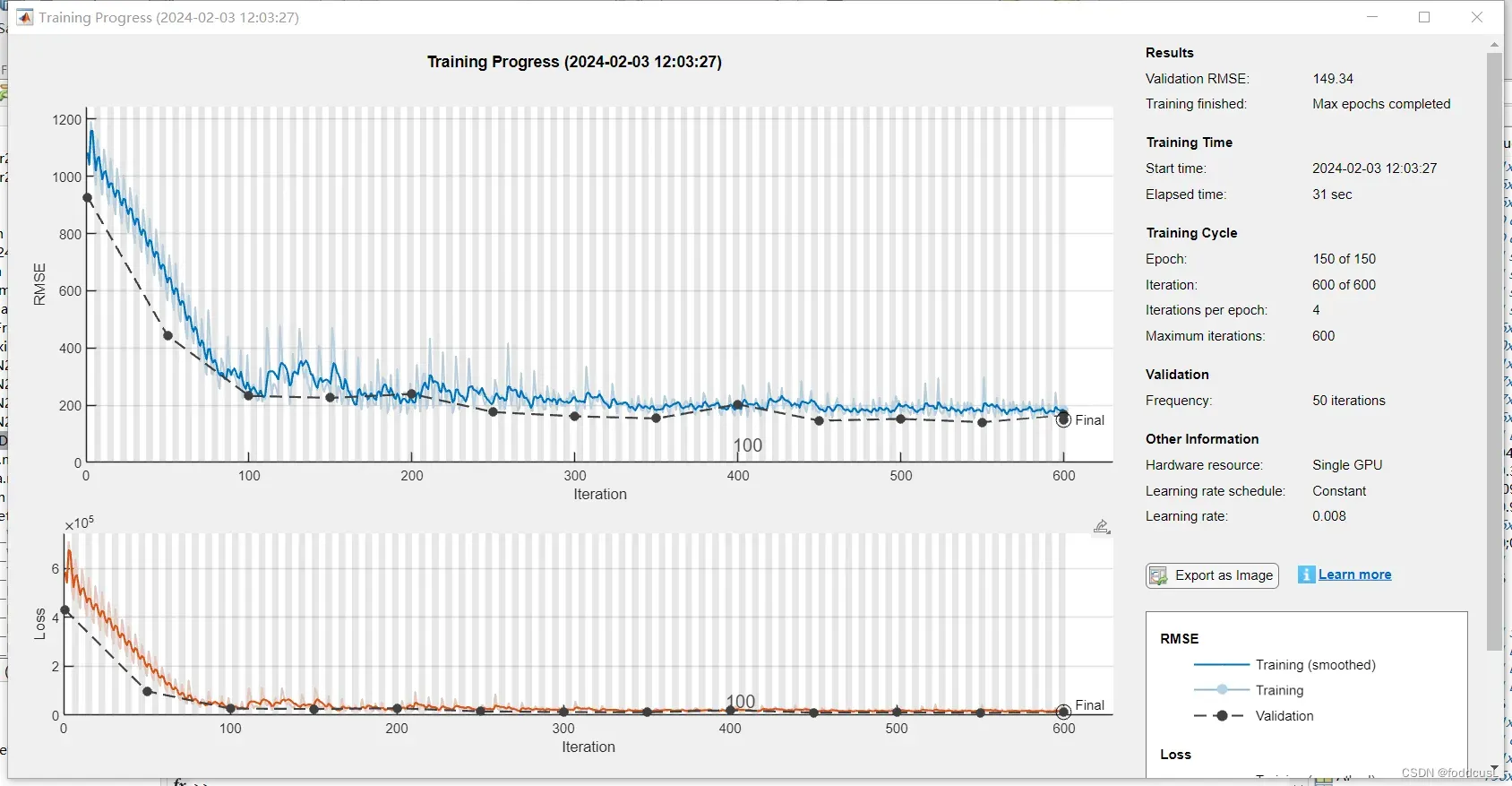
训练过程如下:
训练数据分享
源数据分享:TestData2.mat
链接:https://pan.baidu.com/s/1B1o2xB4aUFOFLzZbwT-7aw?pwd=1xe5
提取码:1xe5
训练建议
以个人经验来说,VNet结构最为简单,但是综合表现最差。对于800-3000长度的数据,容量较小的RNet的表现会比ENet好,对于长度超过的3000的一维数据,ENet的表现更好。
关于超参数的设计:首先最小批次minibatch设置小于64会好一点,确保最终结果会比较好,反正一维卷积神经网络训练很快。第二,与图片不同,一维数据常常数值精度比较高(图片一般就uint8或16格式),因此学习率不宜太高,要不表现会有所下降。我自己尝试的比较好的学习率是0.008.总体来说0.015-0.0005之间都OK,0.05以上结果就开始下降了。
其他引用函数
KS数据划分
Kennard-Stone(KS)方法是一种常用于数据集划分的方法,尤其适用于化学计量学等领域。其主要原理是保证训练集中的样本按照空间距离分布均匀。
function [XSelected,XRest,vSelectedRowIndex]=ks(X,Num) %Num=三分之二的数值
%  ks selects the samples XSelected which uniformly distributed in the exprimental data X's space
%  Input
%         X:the matrix of the sample spectra
%         Num:the number of the sample spectra you want select
%  Output
%         XSelected:the sample spectras was sel   ected from the X
%         XRest:the sample spectras remain int the X after select
%         vSelectedRowIndex:the row index of the selected sample in the X matrix
%  Programmer: zhimin zhang @ central south university on oct 28 ,2007


%%%%%%%%%%%%%%%%%%%%%%%%%%%%%%%%%%%%%%%%%%%%%%%%%%%%%%%%%%%%%%%%%%%
% start of the kennard-stone step one
%%%%%%%%%%%%%%%%%%%%%%%%%%%%%%%%%%%%%%%%%%%%%%%%%%%%%%%%%%%%%%%%%%%

[nRow,nCol]=size(X); % obtain the size of the X matrix
mDistance=zeros(nRow,nRow); %dim a matrix for the distance storage
vAllofSample=1:nRow;

for i=1:nRow-1

    vRowX=X(i,:); % obtain a row of X

    for j=i+1:nRow

        vRowX1=X(j,:); % obtain another row of X
        mDistance(i,j)=norm(vRowX-vRowX1); % calc the Euclidian distance


    end

end


[vMax,vIndexOfmDistance]=max(mDistance);

[nMax,nIndexofvMax]=max(vMax);


%vIndexOfmDistance(1,nIndexofvMax)
%nIndexofvMax
vSelectedSample(1)=nIndexofvMax;
vSelectedSample(2)=vIndexOfmDistance(nIndexofvMax);
%%%%%%%%%%%%%%%%%%%%%%%%%%%%%%%%%%%%%%%%%%%%%%%%%%%%%%%%%%%%%%%%%%
% end of the kennard-stone step one
%%%%%%%%%%%%%%%%%%%%%%%%%%%%%%%%%%%%%%%%%%%%%%%%%%%%%%%%%%%%%%%%%%%


%%%%%%%%%%%%%%%%%%%%%%%%%%%%%%%%%%%%%%%%%%%%%%%%%%%%%%%%%%%%%%%%%%
% start of the kennard-stone step two
%%%%%%%%%%%%%%%%%%%%%%%%%%%%%%%%%%%%%%%%%%%%%%%%%%%%%%%%%%%%%%%%%%%

for i=3:Num
    vNotSelectedSample=setdiff(vAllofSample,vSelectedSample);
    vMinDistance=zeros(1,nRow-i + 1);


    for j=1:(nRow-i+1)
        nIndexofNotSelected=vNotSelectedSample(j);
        vDistanceNew = zeros(1,i-1);

        for k=1:(i-1)
            nIndexofSelected=vSelectedSample(k);
            if(nIndexofSelected<=nIndexofNotSelected)
                vDistanceNew(k)=mDistance(nIndexofSelected,nIndexofNotSelected);
            else
                vDistanceNew(k)=mDistance(nIndexofNotSelected,nIndexofSelected);
            end
        end

        vMinDistance(j)=min(vDistanceNew);
    end

    [nUseless,nIndexofvMinDistance]=max(vMinDistance);
    vSelectedSample(i)=vNotSelectedSample(nIndexofvMinDistance);
end

%%%%%%%%%%%%%%%%%%%%%%%%%%%%%%%%%%%%%%%%%%%%%%%%%%%%%%%%%%%%%%%%%%
%%%%% end of the kennard-stone step two
%%%%%%%%%%%%%%%%%%%%%%%%%%%%%%%%%%%%%%%%%%%%%%%%%%%%%%%%%%%%%%%%%%%


%%%%%%%%%%%%%%%%%%%%%%%%%%%%%%%%%%%%%%%%%%%%%%%%%%%%%%%%%%%%%%%%%%
%%%%% start of export the result
%%%%%%%%%%%%%%%%%%%%%%%%%%%%%%%%%%%%%%%%%%%%%%%%%%%%%%%%%%%%%%%%%%%
vSelectedRowIndex=vSelectedSample;

for i=1:length(vSelectedSample)

    XSelected(i,:)=X(vSelectedSample(i),:);
end

vNotSelectedSample=setdiff(vAllofSample,vSelectedSample);
for i=1:length(vNotSelectedSample)

    XRest(i,:)=X(vNotSelectedSample(i),:);
end

%%%%%%%%%%%%%%%%%%%%%%%%%%%%%%%%%%%%%%%%%%%%%%%%%%%%%%%%%%%%%%%%%%
%%%%% end of export the result
%%%%%%%%%%%%%%%%%%%%%%%%%%%%%%%%%%%%%%%%%%%%%%%%%%%%%%%%%%%%%%%%%%%
参考文献
卷积神经网络的紫外-可见光谱水质分类方法 (wanfangdata.com.cn)
光谱技术结合水分校正与样本增广的棉田土壤盐分精准反演 (tcsae.org)
版权声明:本文为博主作者:foddcusL原创文章,版权归属原作者,如果侵权,请联系我们删除!
原文链接:https://blog.csdn.net/m0_47787372/article/details/135975924