【Python搜索算法】广度优先搜索（BFS）算法原理详解与应用，示例+代码

目录

1 广度优先搜索    

2 应用示例

2.1 迷宫路径搜索

2.2 社交网络中的关系度排序

2.3 查找连通区域

1 广度优先搜索    

        广度优先搜索（Breadth-First Search，BFS）是一种图遍历算法，用于系统地遍历或搜索图（或树）中的所有节点。BFS的核心思想是从起始节点开始，首先访问其所有相邻节点，然后逐层向外扩展，逐一访问相邻节点的相邻节点，以此类推。这意味着BFS会优先探索距离起始节点最近的节点，然后再逐渐扩展到距离更远的节点。BFS通常用于查找最短路径、解决迷宫问题、检测图是否连通以及广泛的图问题。

BFS算法的步骤如下：

1. 初始化：选择一个起始节点，将其标记为已访问，并将其放入队列中（作为起始节点）。

2. 进入循环：重复以下步骤，直到队列为空。 a. 从队列中取出一个节点。 b. 访问该节点。 c. 将所有未访问的相邻节点加入队列。 d. 标记已访问的节点，以避免重复访问。

3. 结束循环：当队列为空时，表示已经遍历完整个图。

以下是BFS的算法原理详解和一个应用示例：

算法原理：

        BFS的工作原理是通过队列数据结构来管理待访问的节点。它从起始节点开始，然后逐一访问该节点的相邻节点，并将它们加入队列。然后，它从队列中取出下一个节点进行访问，以此类推。这确保了节点按照它们的距离从起始节点逐层遍历，因此BFS可以用于查找最短路径。

        BFS是一个宽度优先的搜索，它在查找最短路径等问题中非常有用。它不会陷入深度过深的路径，因为它会优先探索距离起始节点更近的节点。

2 应用示例

2.1 迷宫路径搜索

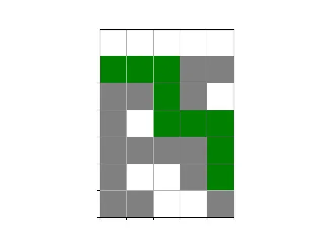
        假设有一个迷宫，其中包含墙壁和通道，您希望找到从起始点到终点的最短路径。BFS是解决这类问题的理想选择。

示例迷宫：

S 0 0 1 1 1
1 1 0 1 0 1
1 0 0 0 0 1
1 1 1 1 0 1
1 0 0 1 0 1
1 1 1 1 1 E

• S 表示起始点
• E 表示终点
• 0 表示可以通过的通道
• 1 表示墙壁

 使用BFS，您可以找到从起始点到终点的最短路径，如下所示：

1. 从起始点 S 开始，将其加入队列。
2. 逐层遍历节点，首先访问距离 S 最近的节点。
3. 在每一步中，将所有可以通过的相邻节点加入队列，同时标记已访问的节点。
4. 继续这个过程，直到到达终点 E。

BFS会优先探索距离 S 最近的通道，因此它会找到从 S 到 E 的最短路径。在上面的迷宫中，BFS将找到一条最短路径，经过标有数字 0 的通道，最终到达终点 E。这是BFS在寻找最短路径问题中的一个实际应用示例。

示例：

import matplotlib.pyplot as plt
from collections import deque


def bfs_shortest_path(maze, start, end):
    # 定义四个方向移动的偏移量，分别是上、下、左、右
    directions = [(-1, 0), (1, 0), (0, -1), (0, 1)]
    rows, cols = len(maze), len(maze[0])

    # 创建队列用于BFS
    queue = deque([(start, [start])])
    visited = set()

    while queue:
        (x, y), path = queue.popleft()
        visited.add((x, y))

        if (x, y) == end:
            return path  # 找到了最短路径

        for dx, dy in directions:
            new_x, new_y = x + dx, y + dy

            if 0 <= new_x < rows and 0 <= new_y < cols and maze[new_x][new_y] == 0 and (new_x, new_y) not in visited:
                new_path = path + [(new_x, new_y)]
                queue.append(((new_x, new_y), new_path))

    return None  # 没有找到路径

def draw_maze(maze, path=None):
    rows, cols = len(maze), len(maze[0])

    # 创建一个图形对象
    fig, ax = plt.subplots()

    # 绘制迷宫
    for x in range(rows):
        for y in range(cols):
            if maze[x][y] == 0:
                ax.add_patch(plt.Rectangle((y, -x - 1), 1, 1, facecolor="white"))
            else:
                ax.add_patch(plt.Rectangle((y, -x - 1), 1, 1, facecolor="gray"))

    # 绘制路径（如果存在）
    if path:
        for x, y in path:
            ax.add_patch(plt.Rectangle((y, -x - 1), 1, 1, facecolor="green"))

    # 设置坐标轴
    ax.set_aspect("equal")
    ax.set_xticks(range(cols))
    ax.set_yticks(range(-rows, 0))
    ax.set_xticklabels([])
    ax.set_yticklabels([])

    plt.grid(True)
    plt.show()


# 示例迷宫，0表示通道，1表示墙壁
maze = [
    [0, 0, 0, 1, 1, 1],
    [1, 1, 0, 1, 0, 1],
    [1, 0, 0, 0, 0, 1],
    [1, 1, 1, 1, 0, 1],
    [1, 0, 0, 1, 0, 0],
    [1, 1, 0, 0, 1, 0]
]

start = (0, 0)  # 起始点
end = (5, 5)  # 终点

path = bfs_shortest_path(maze, start, end)

draw_maze(maze, path)

2.2 社交网络中的关系度排序

        广度优先搜索（BFS）的排序应用示例之一是使用它在无权图中查找最短路径。在前面的示例中，我们已经展示了如何使用BFS查找迷宫中的最短路径。这是BFS的一个典型应用示例。

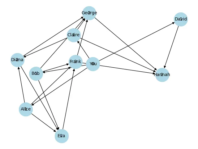
        另一个排序应用示例是社交网络中的关系度排序。在社交网络中，您可以使用BFS来确定您与其他用户之间的关系度，即您与其他用户之间的最短路径，或者共同的朋友数量。以下是一个简单的示例：

        假设您有一个社交网络，其中用户之间的关系用图表示，其中节点代表用户，边代表用户之间的关系。您想知道您与其他用户之间的关系度，并按关系度对用户进行排序。

import networkx as nx
import matplotlib.pyplot as plt
from collections import deque

# 创建一个复杂的社交网络图
social_network = {
    'You': ['Alice', 'Bob', 'Claire', 'David'],
    'Alice': ['Diana', 'Eva', 'Frank'],
    'Bob': ['Eva', 'Frank', 'George'],
    'Claire': ['Diana', 'George', 'Hannah'],
    'David': ['Hannah'],
    'Diana': ['Eva', 'George'],
    'Eva': ['Frank'],
    'Frank': ['George', 'Hannah'],
    'George': ['Hannah'],
    'Hannah': [],
}

def bfs_relationship_degree(graph, start):
    visited = set()
    queue = deque([(start, 0)])  # 用于存储节点和关系度

    relationship_degree = {}  # 存储关系度

    while queue:
        node, degree = queue.popleft()

        if node not in visited:
            visited.add(node)
            relationship_degree[node] = degree

            for friend in graph[node]:
                if friend not in visited:
                    queue.append((friend, degree + 1))

    return relationship_degree

# 使用BFS查找关系度
your_name = 'You'
relationship_degree = bfs_relationship_degree(social_network, your_name)

# 创建一个有向图
G = nx.DiGraph()

# 添加节点和边
for user, degree in relationship_degree.items():
    G.add_node(user, degree=degree)

for user in social_network:
    for friend in social_network[user]:
        G.add_edge(user, friend)

# 绘制图形
pos = nx.spring_layout(G, seed=42)
labels = nx.get_node_attributes(G, 'degree')
nx.draw(G, pos, with_labels=True, node_size=1000, node_color='lightblue', font_size=10, font_color='black')
nx.draw_networkx_labels(G, pos, labels, font_size=10, font_color='black')
plt.title("复杂社交网络图")
plt.show()

# 输出排序结果
sorted_users = sorted(relationship_degree.items(), key=lambda x: x[1])
for user, degree in sorted_users:
    print(f'{user}: 关系度 {degree}')

输出：

 输出：

You: 关系度 0
Alice: 关系度 1
Bob: 关系度 1
Claire: 关系度 1
David: 关系度 1
Diana: 关系度 2
Eva: 关系度 2
Frank: 关系度 2
George: 关系度 2
Hannah: 关系度 2

 这段代码的目的是使用广度优先搜索（BFS）算法来查找社交网络中您（’You’）与其他用户之间的关系度，并绘制社交网络图。

1. 首先，定义了一个复杂的社交网络图，其中包括不同用户之间的关系。这个社交网络图存储在 social_network 字典中。

2. bfs_relationship_degree 函数实现了BFS算法来查找您与其他用户之间的关系度。它从您开始，逐层查找与您相连接的用户，计算它们之间的关系度。结果存储在 relationship_degree 字典中。

3. 创建一个有向图（DiGraph） G 以绘制社交网络图。

4. 添加节点和边到图 G，其中节点代表用户，边代表用户之间的关系。此时，节点的颜色和大小被设置为 lightblue 和 1000，并且边的颜色为 gray。

5. 使用 NetworkX 提供的布局算法 spring_layout 来确定节点的位置。

6. 绘制图形，包括节点和边，以及节点上的标签。

7. 输出用户的关系度排序结果，按照从您（’You’）到其他用户的关系度进行排序。

运行该代码将绘制出社交网络图，并输出用户的关系度排序结果。这可以帮助您可视化您与其他用户之间的关系，并查看谁与您更亲近。

2.3 查找连通区域

        在图像处理中，连通区域是由相邻像素组成的区域，具有相似的特性（如颜色或灰度）。BFS可以用来查找和标记这些连通区域。

import cv2
import numpy as np

# 读取图像
image = cv2.imread('img.jpg', 0)  # 以灰度模式读取图像
ret, binary_image = cv2.threshold(image, 127, 255, cv2.THRESH_BINARY)

# 创建一个与图像大小相同的标记图
height, width = binary_image.shape
markers = np.zeros((height, width), dtype=np.int32)

# 定义一个颜色映射
color_map = {
    1: (0, 0, 255),  # 红色
    2: (0, 255, 0),  # 绿色
    3: (255, 0, 0),  # 蓝色
    4: (0, 255, 255),  # 黄色
    # 您可以根据需要添加更多颜色
}

# 连通区域计数
region_count = 0

# 定义8个邻域的偏移
neighbor_offsets = [(-1, -1), (-1, 0), (-1, 1), (0, -1), (0, 1), (1, -1), (1, 0), (1, 1)]

# 开始查找连通区域
for y in range(height):
    for x in range(width):
        if binary_image[y, x] == 255 and markers[y, x] == 0:
            region_count += 1
            markers[y, x] = region_count
            queue = [(y, x)]

            while queue:
                current_y, current_x = queue.pop(0)

                for dy, dx in neighbor_offsets:
                    ny, nx = current_y + dy, current_x + dx

                    if 0 <= ny < height and 0 <= nx < width and binary_image[ny, nx] == 255 and markers[ny, nx] == 0:
                        markers[ny, nx] = region_count
                        queue.append((ny, nx))

# 将连通区域标记为不同颜色
result_image = np.zeros((height, width, 3), dtype=np.uint8)
for y in range(height):
    for x in range(width):
        if markers[y, x] > 0:
            result_image[y, x] = color_map[markers[y, x]]

# 显示结果图像
cv2.imshow('Connected Components', result_image)
cv2.waitKey(0)
cv2.destroyAllWindows()

         这段代码首先读取了一个灰度图像（也可以使用彩色图像），将其转换为二值图像。然后，它使用BFS算法查找连通区域，对不同的连通区域进行标记，并将它们标记为不同的颜色。最后，它显示带有标记的结果图像。