使用 NLP 和机器学习预测假新闻 | Scikit-学习 |手套 |喀拉斯 |长短期记忆体

在 Kaggle 的假新闻数据集上使用 Python 应用传统机器学习和深度学习技术的简单指南。它还简要包括文章的文本和文体分析。

假新闻数据集是 Kaggle 上可用的经典文本分析数据集之一。它由来自不同作者的真假文章标题和文本组成。在本文中，我使用传统的机器学习方法和深度学习完成了整个文本分类过程。[0]

Getting Started

我首先从 Google Colab 上的 Kaggle 下载数据集。

# Upload Kaggle json

!pip install -q kaggle
!pip install -q kaggle-cli
!mkdir -p ~/.kaggle
!cp "/content/drive/My Drive/Kaggle/kaggle.json" ~/.kaggle/ # Mount GDrive
!cat ~/.kaggle/kaggle.json 
!chmod 600 ~/.kaggle/kaggle.json
!kaggle competitions download -c fake-news -p dataset
!unzip /content/dataset/train.csv.zip
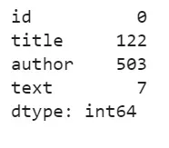
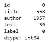
!unzip /content/dataset/test.csv.zip

接下来，我读取了 DataFrame 并检查了其中的空值。在总共 20800 行中，文本文章中有 7 个空值，标题为 122，作者为 503，我决定删除这些行。对于测试数据，我用空白填充它们。

train_df = pd.read_csv('/content/train.csv', header=0)
test_df = pd.read_csv('/content/test.csv', header=0)
print(train_df.isna().sum())
print(test_df.isna().sum())
train_df.dropna(axis=0, how='any',inplace=True)
test_df = test_df.fillna(' ')

此外，我还检查了数据集中“假”和“真”新闻的分布。通常，我在导入 matplotlib 时为笔记本上的所有绘图设置 rcParams。

import matplotlib.pyplot as plt
from matplotlib import rcParams
plt.rcParams['figure.figsize'] = [10, 10]
import seaborn as sns
sns.set_theme(style="darkgrid")

sns.countplot(x='label', data=train_df, palette='Set3')
plt.show()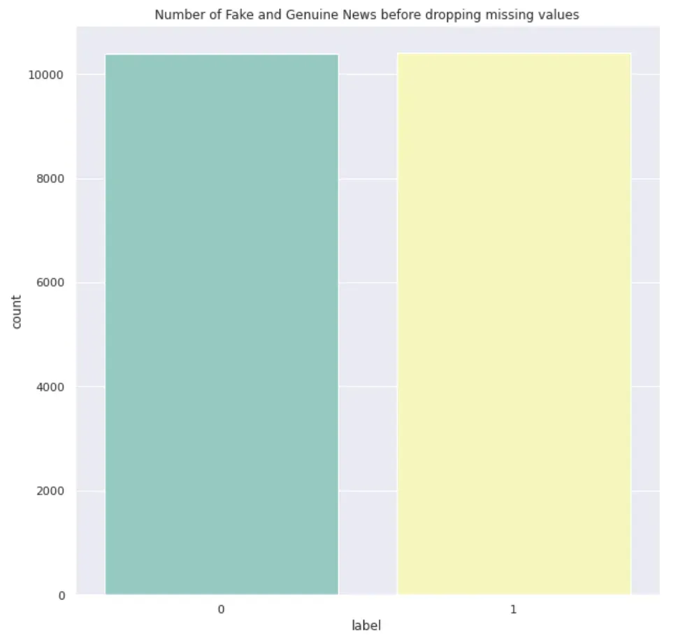

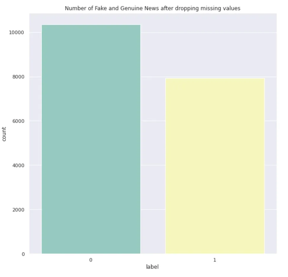
真假新闻的比例从 1:1 变为 4:5。

接下来，我决定看下面的文章长度——

train_df['raw_text_length'] = train_df['text'].apply(lambda x: len(x))
sns.boxplot(y='raw_text_length', x='label', data=train_df, palette="Set3")
plt.show()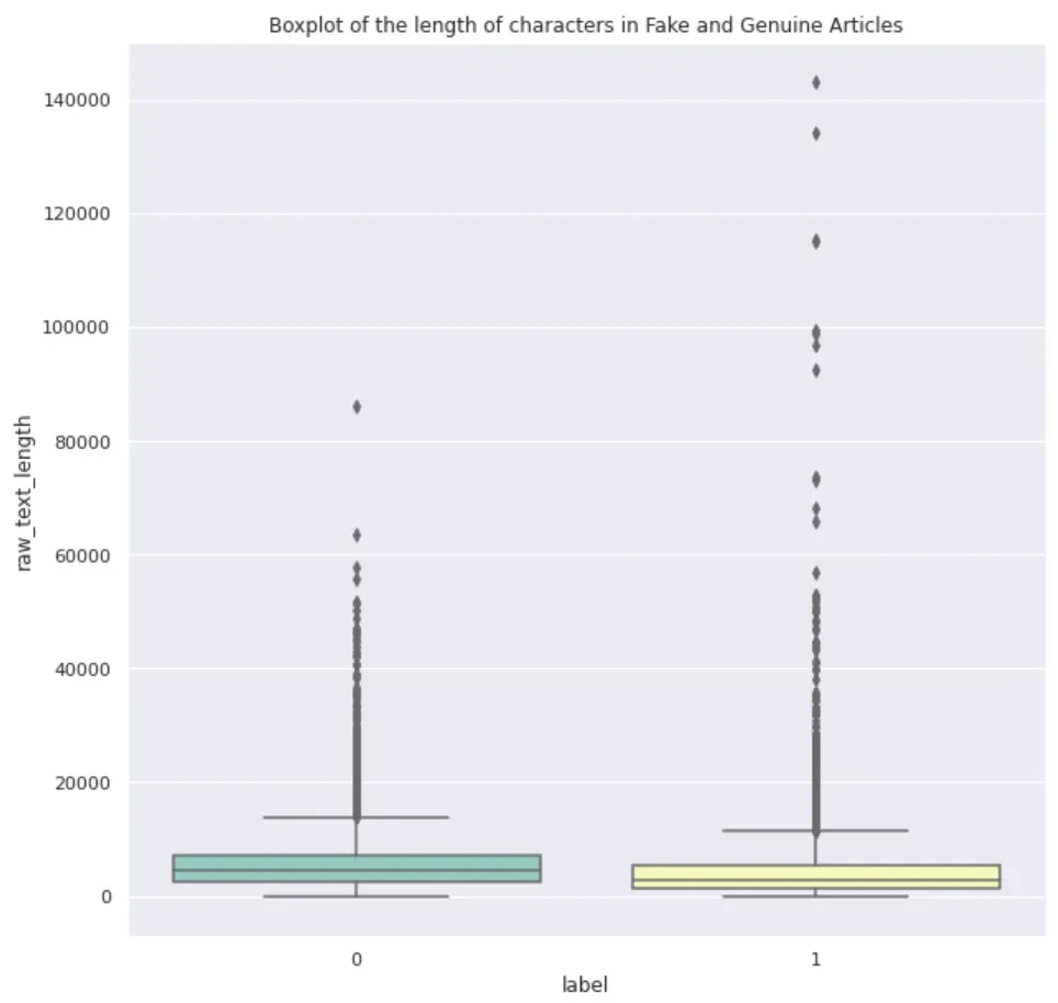

可以看出，假文章的中值长度较低，但也有大量异常值。两者的长度都为零。

可以看出，它们从 0 开始，这是令人担忧的。当我使用 .describe() 查看数字时，它实际上是从 1 开始的。所以我看了看这些文字，发现它们是空白的。显而易见的答案是剥离和下降长度为零。我检查了零长度文本的总数是 74。

train_df['text'] = train_df['text'].str.strip()
# Recalculate the length
train_df['raw_text_length'] = train_df['text'].apply(lambda x: len(x))
print(len(train_df[train_df['raw_text_length']==0]))

我决定重新开始。因此，我将用空白填充所有 nan，然后将它们剥离，然后删除零长度文本，这应该可以很好地开始预处理。以下是本质上处理缺失值的新代码。数据最终的形状为(20684, 6)，即包含20684行，仅比20800少116。

train_df = pd.read_csv('/content/train.csv', header=0)
train_df = train_df.fillna(' ')
train_df['text'] = train_df['text'].str.strip()
train_df['raw_text_length'] = train_df['text'].apply(lambda x: len(x))
print(len(train_df[train_df['raw_text_length']==0]))
print(train_df.isna().sum())
train_df = train_df[train_df['raw_text_length'] > 0]
print(train_df.shape)
print(train_df.isna().sum())

# Visualize the target's distribution
sns.countplot(x='label', data=train_df, palette='Set3')
plt.title("Number of Fake and Genuine News after dropping missing values")
plt.show()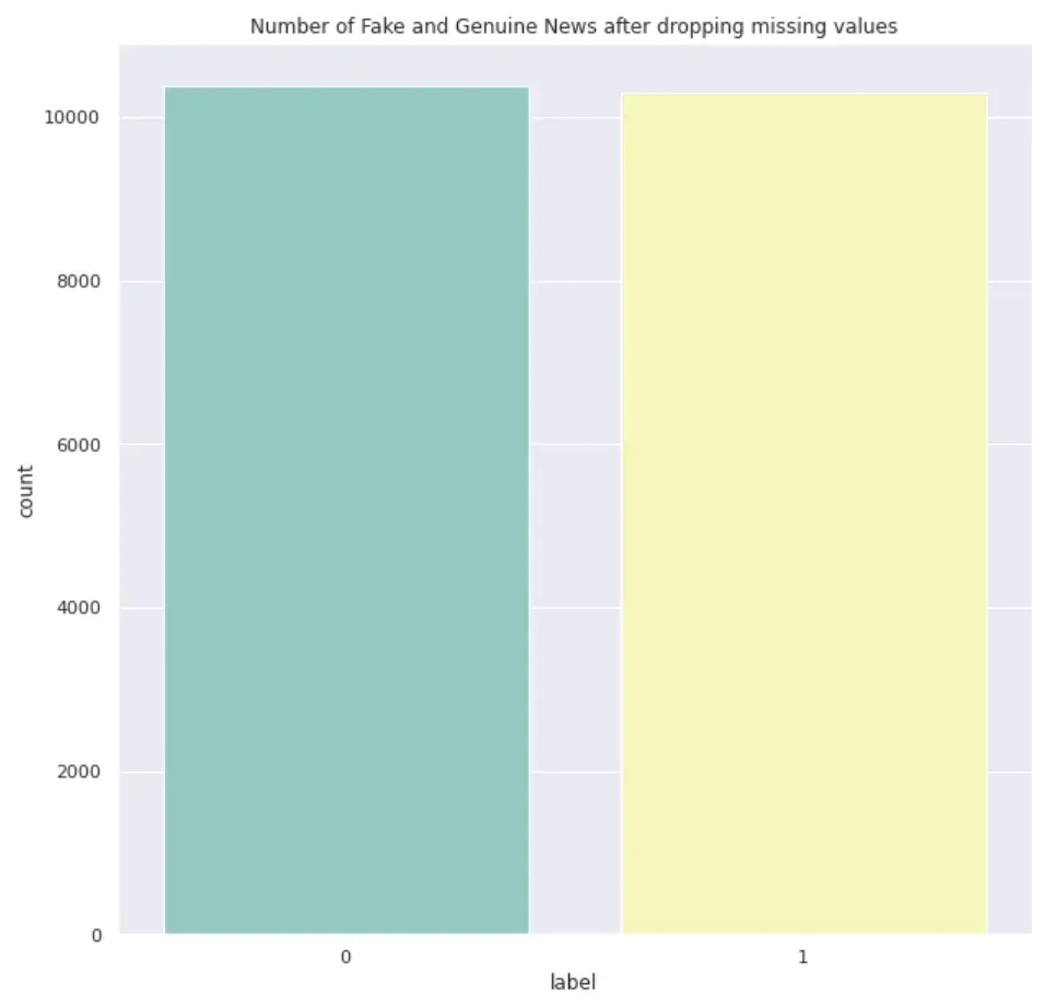

之后出现了更多的文本长度为个位数或低至 10。它们看起来更像是评论而不是正确的文本。我将暂时保留它们并继续下一步。

Text Preprocessing

因此，在我开始进行文本预处理之前，我实际上查看了拥有假文章和真文章的作者的重叠数量。换句话说，获得作者的信息会有所帮助吗？我发现有3838位作者，其中2225位是真实的，1618位是假新闻的作者。其中5位作者为真假新闻作者。

gen_news_authors = set(list(train_df[train_df['label']==0]['author'].unique()))
fake_news_authors = set(list(train_df[train_df['label']==1]['author'].unique()))
overlapped_authors = gen_news_authors.intersection(fake_news_authors)
print("Number of distinct authors with genuine articles: {}", len(gen_news_authors))
print("Number of distinct authors with fake articles: {}", len(fake_news_authors))
print("Number of distinct authors with both genuine and fake: {}", len(overlapped_authors))

从预处理开始，我最初选择直接按空白分割并扩大收缩。但是，由于某些（我想是斯拉夫语）其他语言文本，这已经产生了错误。因此，在第一步中，我使用正则表达式仅保留拉丁字符、数字和空格。然后，扩展收缩，然后转换为小写。这是因为诸如 ive 之类的收缩转换为 I have。因此，在扩大收缩之后转换为小写。完整代码如下：

def preprocess_text(x):
  cleaned_text = re.sub(r'[^a-zA-Z\d\s\']+', '', x)
  word_list = []
  for each_word in cleaned_text.split(' '):
    try:
      word_list.append(contractions.fix(each_word).lower())
    except:
      print(x)
  return " ".join(word_list)
  
text_cols = ['text', 'title', 'author']
for col in text_cols:
  print("Processing column: {}".format(col))
  train_df[col] = train_df[col].apply(lambda x: preprocess_text(x))
  test_df[col] = test_df[col].apply(lambda x: preprocess_text(x)) 

一旦完成，就完成常规单词标记化，然后删除停用词。

for col in text_cols:
    print("Processing column: {}".format(col))
    train_df[col] = train_df[col].apply(word_tokenize)
    test_df[col] = test_df[col].apply(word_tokenize)

for col in text_cols:
    print("Processing column: {}".format(col))
    train_df[col] = train_df[col].apply(
        lambda x: [each_word for each_word in x if each_word not in stopwords])
    test_df[col] = test_df[col].apply(
        lambda x: [each_word for each_word in x if each_word not in stopwords])

Text Analysis

现在数据已经准备好了，我打算使用 wordcloud 查看常用词。为了做到这一点，我首先将所有标记化的文本加入到单独列中的字符串中，因为稍后将在模型训练时使用它们。

# since count vectorizer expects strings

train_df['text_joined'] = train_df['text'].apply(lambda x: " ".join(x))
test_df['text_joined'] = test_df['text'].apply(lambda x: " ".join(x))

接下来，根据标签，创建一个包含所有文本的字符串并创建 wordcloud，如下所示：

# join all texts in resective labels
all_texts_gen = " ".join(train_df[train_df['label']==0]['text_joined'])
all_texts_fake = " ".join(train_df[train_df['label']==1]['text_joined'])

# Wordcloud for Genuine News
wordcloud = WordCloud(width = 800, height = 800,
                background_color ='white',
                stopwords = stopwords,
                min_font_size = 10).generate(all_texts_gen)                       
plt.imshow(wordcloud)
plt.axis("off")
plt.tight_layout(pad = 0)
plt.show()

# Worldcloud for Fake News
wordcloud = WordCloud(width = 800, height = 800,
                background_color ='white',
                stopwords = stopwords,
                min_font_size = 10).generate(all_texts_fake)                    
plt.imshow(wordcloud)
plt.axis("off")
plt.tight_layout(pad = 0)
  
plt.show()

在假新闻词云中，某些词的出现频率明显高于其他词。在真实新闻的 wordcloud 中，混合了不同的字体大小。相反，在假新闻数据集中，较小的文本在背景中，一些词的使用频率更高。假新闻词云中的中型词较少，或者换句话说，出现频率逐渐减少的情况下存在脱节。频率或高或低。

Stylometric Analysis

文体分析通常被称为对作者风格的分析。我将研究一些文体特征，例如每篇文章的句子数量、一篇文章中每句话的平均单词、每篇文章的平均单词长度以及 POS 标签计数。

每篇文章的句子数

为了得到这个，我需要原始数据集，因为我丢失了 train_df 中的句子信息。因此，我将实际数据的副本保存在 orginal_train_df 中，用于将句子转换为序列。

from nltk import sent_tokenize
original_train_df = train_df.copy() 
original_train_df['sent_tokens'] = original_train_df['text'].apply(sent_tokenize)

接下来，我查看了每个目标类别的句子计数，如下所示：

original_train_df['len_sentence'] = original_train_df['sent_tokens'].apply(len)
sns.boxplot(y='len_sentence', x='label', data=original_train_df, palette="Set3")
plt.title("Boxplot of Number of Sentences in Fake and Genuine Articles")
plt.show()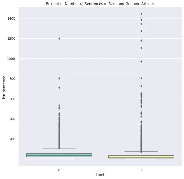

显然，假文章有很多异常值，但 75% 的假文章的句子数低于 50% 的真新闻文章。

一篇文章中每句话的平均字数

在这里，我计算了每篇文章中每个句子的总字数并返回平均值。然后我在箱线图中绘制了计数以可视化它们。

# tokenize words within the sequences
original_train_df['sent_word_tokens'] = original_train_df['sent_tokens'].apply(lambda x: [word_tokenize(each_sentence) for each_sentence in x])

# Clean the punctuations
def get_seq_tokens_cleaned(seq_tokens):
  no_punc_seq = [each_seq.translate(str.maketrans('', '', string.punctuation)) for each_seq in seq_tokens]
  sent_word_tokens = [word_tokenize(each_sentence) for each_sentence in no_punc_seq]
  return sent_word_tokens

# Count the avg number of words in each sentence
def get_average_words_in_sent(seq_word_tokens):
  return np.mean([len(seq) for seq in seq_word_tokens])

original_train_df['sent_word_tokens'] = original_train_df['sent_tokens'].apply(lambda x: get_seq_tokens_cleaned(x))
original_train_df['avg_words_per_sent'] = original_train_df['sent_word_tokens'].apply(lambda x: get_average_words_in_sent(x))

sns.boxplot(y='avg_words_per_sent', x='label', data=original_train_df, palette="Set3")
plt.title("Boxplot of the Average Number of Words per Sentence in Fake and Genuine Articles")
plt.show()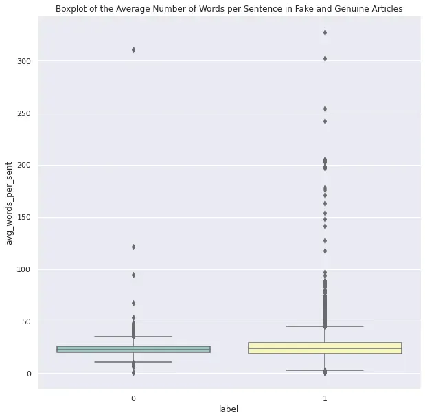

可以看出，平均而言，虚假文章比真实文章更冗长。

每篇文章的平均字长

这是一篇文章的平均字长。在箱线图中，很明显假文章的平均字长更高。

def get_average_word_length(seq_word_tokens):
  return np.mean([len(word) for seq in seq_word_tokens for word in seq])

original_train_df['avg_word_length'] = original_train_df['sent_word_tokens'].apply(lambda x: get_average_words_in_sent(x))

sns.boxplot(y='avg_word_length', x='label', data=original_train_df, palette="Set3")
plt.title("Boxplot of the Average Length of Words per Article in Fake and Genuine Articles")
plt.show()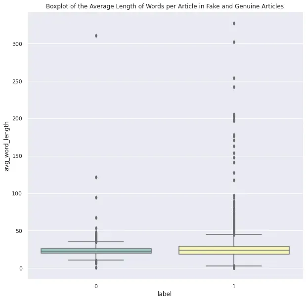

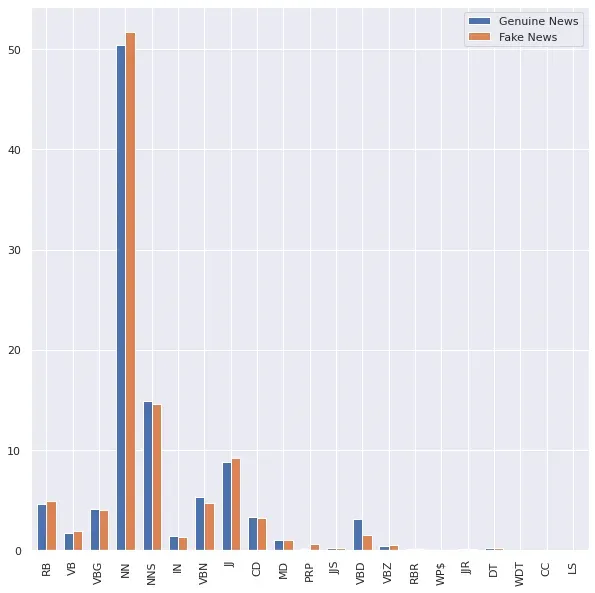
POS Tag Counts

接下来，我尝试查看 Fake vs Genuine 文章中的词性 (POS) 组合。我只在遍历每篇文章时将单词的 POS 存储到一个列表中，将各自的 POS 计数放入一个 DataFrame 中，并使用条形图显示 Fake 和 News 文章中 POS 标签的百分比组合。两篇文章中的名词都高得多。一般来说，除了虚假新闻中过去时动词的百分比是真实新闻的一半之外，没有明显的模式。除此之外，所有其他 POS 类型在假货和真货中几乎相等。

all_tokenized_gen = [a for b in train_df[train_df['label']==0]['text'].tolist() for a in b]
all_tokenized_fake = [a for b in train_df[train_df['label']==1]['text'].tolist() for a in b]

def get_post_tags_list(tokenized_articles):
  all_pos_tags = []
  for word in tokenized_articles:
    pos_tag = nltk.pos_tag([word])[0][1]
    all_pos_tags.append(pos_tag)
  return all_pos_tags
    
all_pos_tagged_word_gen = get_post_tags_list(all_tokenized_gen)
all_pos_tagged_word_fake = get_post_tags_list(all_tokenized_fake)

pritn(all_pos_tagged_word_gen[:5])
print(all_pos_tagged_word_fake[:5])

gen_pos_df = pd.DataFrame(dict(Counter(all_pos_tagged_word_gen)).items(), columns=['Pos_tag', 'Genuine News'])
fake_pos_df = pd.DataFrame(dict(Counter(all_pos_tagged_word_fake)).items(), columns=['Pos_tag', 'Fake News'])
pos_df = gen_pos_df.merge(fake_pos_df, on='Pos_tag')

# Make percentage for comparison
pos_df['Genuine News'] = pos_df['Genuine News'] * 100 / pos_df['Genuine News'].sum()
pos_df['Fake News'] = pos_df['Fake News'] * 100 / pos_df['Fake News'].sum()
pos_df.head()

# plot a multiple bar chart
pos_df.plot.bar(width=0.7)
plt.xticks(range(0,len(pos_df['Pos_tag'])), pos_df['Pos_tag'])
plt.show()

使用机器学习进行文本分类

Tf-idf 和计数矢量化器

分析完成后，我首先采用了使用计数向量器和词频-逆文档频率或 Tf-idf 的常规方法。代码中配置的 Count Vectorizer 也会生成二元组。使用 CountVectorizer() 以矩阵的形式获得它们出现的计数，然后将该字数矩阵转换为标准化的词频 (tf-idf) 表示。在这里，我使用了 smooth=False，以避免零除错误。通过提供 smooth=False，我基本上是在文档频率上加一，因为它是 idf 计算公式中的分母，如下所示 –[0]

idf(t) = log [ n / (df(t) + 1) ]

train_df['text_joined'] = train_df['text'].apply(lambda x: " ".join(x))
test_df['text_joined'] = test_df['text'].apply(lambda x: " ".join(x))

count_vectorizer = CountVectorizer(ngram_range=(1, 2))
tf_idf_transformer = TfidfTransformer(smooth_idf=False)

# fit and transform train data to count vectorizer
count_vectorizer.fit(train_df['text_joined'].values)
count_vect_train = count_vectorizer.transform(train_df['text_joined'].values)

# fit the counts vector to tfidf transformer
tf_idf_transformer.fit(count_vect_train)
tf_idf_train = tf_idf_transformer.transform(count_vect_train)

# Transform the test data as well
count_vect_test = count_vectorizer.transform(test_df['text_joined'].values)
tf_idf_test = tf_idf_transformer.transform(count_vect_test)

# Train test split
X_train, X_test, y_train, y_test = train_test_split(tf_idf_train, target, random_state=0)

使用默认配置进行基准测试

接下来，我打算使用默认配置训练模型，并挑选出性能最好的模型以供以后调整。为此，我遍历了一个列表并将所有性能指标保存到另一个 DataFrame 和列表中的模型中。

df_perf_metrics = pd.DataFrame(columns=['Model', 'Accuracy_Training_Set', 'Accuracy_Test_Set', 'Precision', 'Recall', 'f1_score'])
df_perf_metrics = pd.DataFrame(columns=[
    'Model', 'Accuracy_Training_Set', 'Accuracy_Test_Set', 'Precision',
    'Recall', 'f1_score', 'Training Time (secs'
])

# list to retain the models to use later for test set predictions
models_trained_list = []

def get_perf_metrics(model, i):
    # model name
    model_name = type(model).__name__
    # time keeping
    start_time = time.time()
    print("Training {} model...".format(model_name))
    # Fitting of model
    model.fit(X_train, y_train)
    print("Completed {} model training.".format(model_name))
    elapsed_time = time.time() - start_time
    # Time Elapsed
    print("Time elapsed: {:.2f} s.".format(elapsed_time))
    # Predictions
    y_pred = model.predict(X_test)
    # Add to ith row of dataframe - metrics
    df_perf_metrics.loc[i] = [
        model_name,
        model.score(X_train, y_train),
        model.score(X_test, y_test),
        precision_score(y_test, y_pred),
        recall_score(y_test, y_pred),
        f1_score(y_test, y_pred), "{:.2f}".format(elapsed_time)
    ]
    # keep a track of trained models
    models_trained_list.append(model)
    print("Completed {} model's performance assessment.".format(model_name))

我使用了逻辑回归、多项朴素贝叶斯、决策树、随机森林、梯度提升和 Ada Boost 分类器。 MultinomialNB 的精度是所有中最好的，但由于召回分数差，f1-score 不稳定。事实上，召回率是最差的，为 68%。结果中最好的模型是 Logistic Regression 和 AdaBoost，它们的结果相似。我选择使用逻辑回归来节省训练时间。

models_list = [LogisticRegression(),
               MultinomialNB(),
               RandomForestClassifier(),
               DecisionTreeClassifier(),
               GradientBoostingClassifier(),
               AdaBoostClassifier()]

for n, model in enumerate(models_list):
    get_perf_metrics(model, n)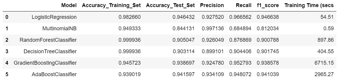

GridSearchCV 用于调整逻辑回归分类器

所以，是时候调整我选择的分类器了。我开始使用更大范围的 max_iter 和 C。然后使用 cv=r 的 GirdSearchCV，即 5 折用于交叉验证，因为标签分布是公平分布的。我使用 f1-score 进行评分，并使用 refit 返回具有最佳 f1-score 的训练模型。[0]

model = LogisticRegression()

max_iter = [100, 200, 500, 1000]
C = [0.1, 0.5, 1, 10, 50, 100]

param_grid = dict(max_iter=max_iter, C=C)

grid = GridSearchCV(estimator=model,
                    param_grid=param_grid,
                    cv=5,
                    scoring=['f1'],
                    refit='f1',
                    verbose=2)

grid_result = grid.fit(X_train, y_train)
print('Best params: ', grid_result.best_params_)

model = grid_result.best_estimator_

y_pred = model.predict(X_test)
print('Accuracy: ', accuracy_score(y_test, y_pred))
print('Precision: ', precision_score(y_test, y_pred))
print('Recall: ', recall_score(y_test, y_pred))
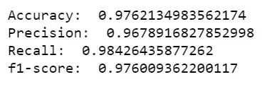
print('f1-score: ', f1_score(y_test, y_pred))

最好的模型具有 97.62% 的准确度和 97.60% 的 f1 分数。对于两者，我们都实现了 4% 的改进。现在，我注意到 max_iter 的最佳值为 100，这是范围的下限，而对于 C，它也是 100，但它是范围的上限。因此，为了适应参数搜索，我使用了 max_iter = 50, 70, 100 和 C = 75, 100, 125。 max_iter=100 和 C=125 有边际改进。所以，我决定保持这个不变，并将 C 的参数搜索从 120 扩大到 150，步长为 10。这次运行的所有性能指标都与起始网格的结果相同。但是，此运行的 C=140 的值。

# Starting out with a range of values
max_iter = [100, 200, 500, 1000]
C = [0.1, 0.5, 1, 10, 50, 100]

# Attempt 2
max_iter = [50, 75, 100]
C = [75, 100, 125]

# Attempt 3
max_iter = [100]
C = [120, 130, 140, 150]

# Final Attempt - Attempt 4
max_iter = [100]
C = [100, 125, 140]

最后一次，我在 max_iter=100 和 C = [100, 125, 140] 上运行网格搜索，其中 C 具有所有运行中的最佳参数。最好的一个是 max_iter=100 和 C=140，我最终将其保存为最佳模型。

这里潜在的未来工作之一是使用 GradientBoost 和 AdaBoost 分类器进行测试，因为它们的性能也很好。在某些情况下，调优后的性能可能会好得多，但出于时间考虑，我会在这里得出结论，因为 Logistic Regression 是 max_iter=100 和 C=140 时性能最好的模型。

我终于把结果上传到了 Kaggle。这个挑战已经有 3 年了，但我有兴趣在这个模型的测试数据上测试分数。

使用 GloVe 和 LSTM 进行文本分类

Data Preparation

为了使用深度学习技术，文本数据必须以原始格式重新加载，因为嵌入会有些不同。在下面的代码中，我处理了缺失值并将文章的标题和作者附加到文章的文本中。

import pandas as pd

train_df = pd.read_csv('fake-news/train.csv', header=0)
test_df = pd.read_csv('fake-news/test.csv', header=0)

train_df = train_df.fillna(' ')
test_df = test_df.fillna(' ')

train_df['all_info'] = train_df['text'] + train_df['title'] + train_df['author']
test_df['all_info'] = test_df['text'] + test_df['title'] + test_df['author']

target = train_df['label'].values

接下来，我使用 Keras API 的 Tokenizer 类对文本进行标记，并使用 oov_token = “” 替换词汇表之外的标记，这实际上是根据词频创建词汇索引。然后我将标记器安装在文本上并将它们转换为整数序列，该序列使用通过拟合标记器创建的词汇索引。最后，由于序列可能有不同的长度，我使用 pad_sequences 在最后使用 padding=post 用零填充它们。因此，根据代码，每个序列的长度预计为 40。最后，我将它们分成训练集和测试集。[0]

from tensorflow.keras.preprocessing.text import Tokenizer
from tensorflow.keras.preprocessing.sequence import pad_sequences

tokenizer = Tokenizer(oov_token = "", num_words=6000)
tokenizer.fit_on_texts(train_df['all_info'])

max_length = 40
vocab_size = 6000

sequences_train = tokenizer.texts_to_sequences(train_df['all_info'])
sequences_test = tokenizer.texts_to_sequences(test_df['all_info'])

padded_train = pad_sequences(sequences_train, padding = 'post', maxlen=max_length)
padded_test = pad_sequences(sequences_test, padding = 'post', maxlen=max_length)

X_train, X_test, y_train, y_test = train_test_split(padded_train, target, test_size=0.2)

print(X_train.shape)
print(y_train.shape)

Binary Classification Model

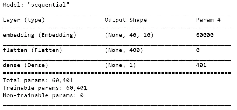
为了创建文本分类模型，我从最简单形式的二元分类模型结构开始，其中第一层是嵌入层，期望嵌入 6000 个词汇大小（在 vocab_size 中指定）的文本，每个序列的长度为 40（因此, input_length=max_length) 并为每个输入序列提供 40 个 10 维向量的输出。接下来，我使用 Flatten 层将形状 (40, 10) 的矩阵展平为单个形状阵列 (400, )。然后，该数组通过 Dense 层产生一维输出，并使用 sigmoid 激活函数产生二元分类。我最初想用这个模型做更多的实验，所以为它创建了一个函数，我也喜欢将层分组到一个函数中作为一种实践。这项工作并不真正需要它。最后，我使用精确度和召回率来编译模型，以便在训练和验证时监控指标。[0][1][2]

def get_simple_model():
  model = Sequential()
  model.add(Embedding(vocab_size, 10, input_length=max_length))
  model.add(Flatten())
  model.add(Dense(1, activation='sigmoid'))
  return model
  
model = get_simple_model()
print(model.summary())

model.compile(loss='binary_crossentropy',
              optimizer='adam', 
              metrics=[tf.keras.metrics.Precision(), tf.keras.metrics.Recall()])

我还使用了提前停止来节省时间，其中有耐性=15，这表示如果在最后 15 个时期内模型没有改进，则停止，并使用模型检查点来存储最好的模型，并且 save_best_only=True。添加了 mode=min 因为我在这里监控损失。

callbacks=[
    keras.callbacks.EarlyStopping(monitor="val_loss", patience=15, 
                                  verbose=1, mode="min", restore_best_weights=True),
    keras.callbacks.ModelCheckpoint(filepath=best_model_file_name, verbose=1, save_best_only=True)
]

现在是时候拟合模型了！

history = model.fit(X_train, 
                    y_train, 
                    epochs=20,
                    validation_data=(X_test, y_test), 
                    callbacks=callbacks)

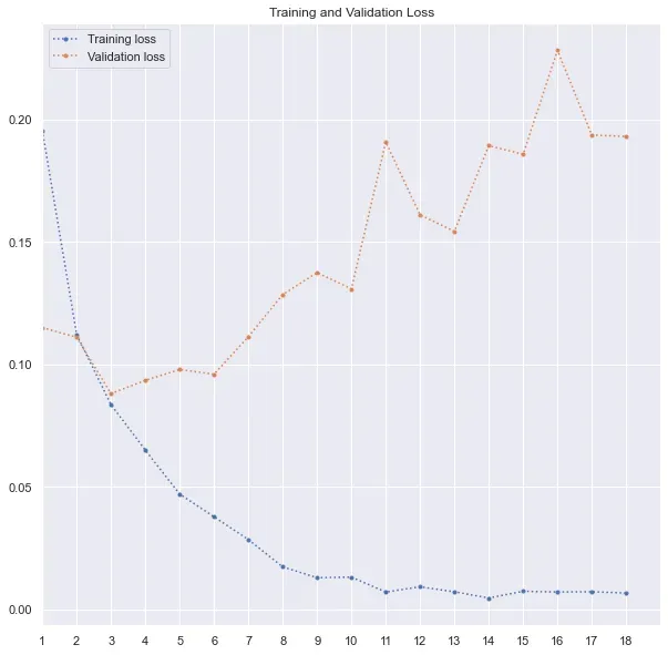
print(history.history.keys())

由于我使用了准确率和召回率以及损失，因此我还可以在这里跟踪准确率和召回率值。如下图所示，验证损失在第 6 个时期最低，然后损失要么停滞不前，要么增加。因此，最好的模型在第 6 轮训练后被保存。很明显，模型是如何过度拟合的，训练损失有所改善，而验证损失在第 6 个 epoch 后增加。

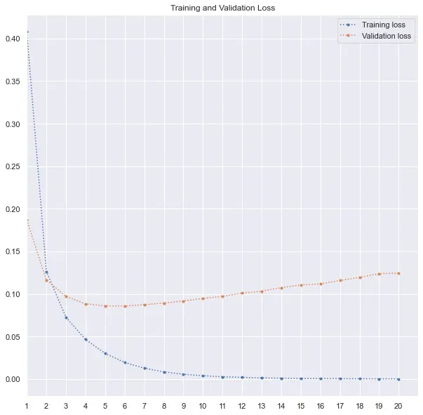
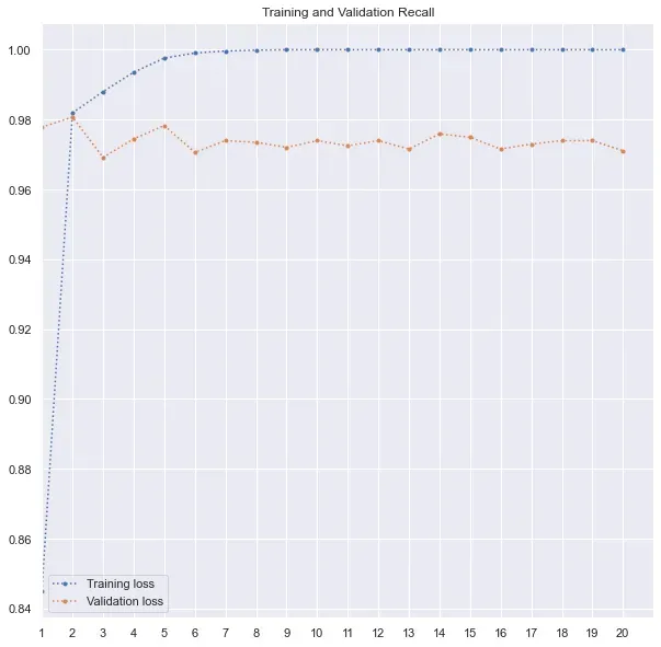
下面是我用来绘制训练和验证损失、精度和召回率的代码。我在 range 函数中使用了 max(history.epoch) + 2，因为 history.epoch 从 0 开始。因此，对于 20 个 epoch，最大值为 19，并且范围将为 max(history.epoch) 生成一个从 1 到 18 的列表）。

# plot training and validation loss

metric_to_plot = "loss"
plt.plot(range(1, max(history.epoch) + 2), history.history[metric_to_plot], ".:", label="Training loss")
plt.plot(range(1, max(history.epoch) + 2), history.history["val_" + metric_to_plot], ".:", label="Validation loss")
plt.title('Training and Validation Loss')
plt.xlim([1,max(history.epoch) + 2])
plt.xticks(range(1, max(history.epoch) + 2))
plt.legend()
plt.show()

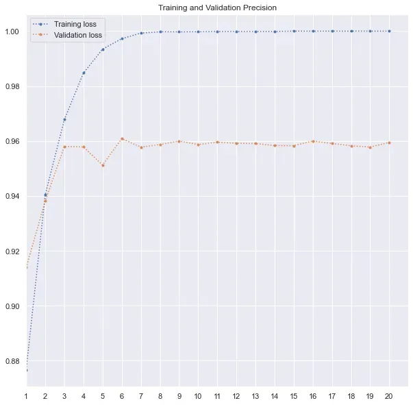
# plot training and validation precision

metric_to_plot = "precision"
plt.plot(range(1, max(history.epoch) + 2), history.history[metric_to_plot], ".:", label="Training loss")
plt.plot(range(1, max(history.epoch) + 2), history.history["val_" + metric_to_plot], ".:", label="Validation loss")
plt.title('Training and Validation Precision')
plt.xlim([1,max(history.epoch) + 2])
plt.xticks(range(1, max(history.epoch) + 2))
plt.legend()
plt.show()

# plot training and validation recall

metric_to_plot = "recall"
plt.plot(range(1, max(history.epoch) + 2), history.history[metric_to_plot], ".:", label="Training loss")
plt.plot(range(1, max(history.epoch) + 2), history.history["val_" + metric_to_plot], ".:", label="Validation loss")
plt.title('Training and Validation Recall')
plt.xlim([1,max(history.epoch) + 2])
plt.xticks(range(1, max(history.epoch) + 2))
plt.legend()
plt.show()

该模型的准确率为 96.6%，f1 分数为 96.6%。我还在 Kaggle 测试数据上测试了这个模型的性能，它还不错，但并不比我之前训练的 Logistic Regression 好。

LSTM

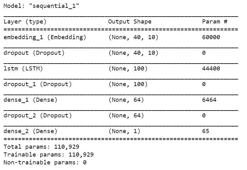
呸！现在让我们将 LSTM 模型拟合到文本数据中。第一层和最后一层是相同的，因为输入和输出是相同的。在这之间，我使用了一个 Dropout 层来过滤掉 30% 的单元，然后进入 100 个单元的 LSTM 层。长短期记忆（LSTM），是一种特殊的 RNN，能够学习长期依赖。他们的专长在于更长时间地记住信息。在使用 LSTM 之后，我使用了另一个 Dropout 层，然后是一个具有 64 个隐藏单元的全连接层，然后是另一个 Dropout 层，最后是另一个具有“Sigmoid”激活函数的单元的全连接层，用于二进制分类。[0][1]

def get_simple_LSTM_model():
  model = Sequential()
  model.add(Embedding(vocab_size, 10, input_length=max_length))
  model.add(Dropout(0.3))
  model.add(LSTM(100))
  model.add(Dropout(0.3))
  model.add(Dense(64, activation='relu'))
  model.add(Dropout(0.3))
  model.add(Dense(1, activation='sigmoid'))
  return model

model = get_simple_LSTM_model()
print(model.summary())

完成后，我按照上一节中概述的相同过程来编译、使用回调并拟合模型。我提供的 epoch 数是 20。但在这种情况下，模型只训练了 16 个 epoch，因为在第一个 epoch 之后的 15 次连续迭代中，验证损失没有任何改善。从下面的图中也可以清楚地看到。验证损失只是在增加，而训练损失由于过度拟合而下降。回想一下我对模型进行编码的回调设置，在停止之前等待 15 个连续 epoch 的验证损失有所改善。

callbacks=[
    keras.callbacks.EarlyStopping(monitor="val_loss", patience=15, 
                                  verbose=1, mode="min", restore_best_weights=True),
    keras.callbacks.ModelCheckpoint(filepath=best_model_file_name, verbose=1, save_best_only=True)
]

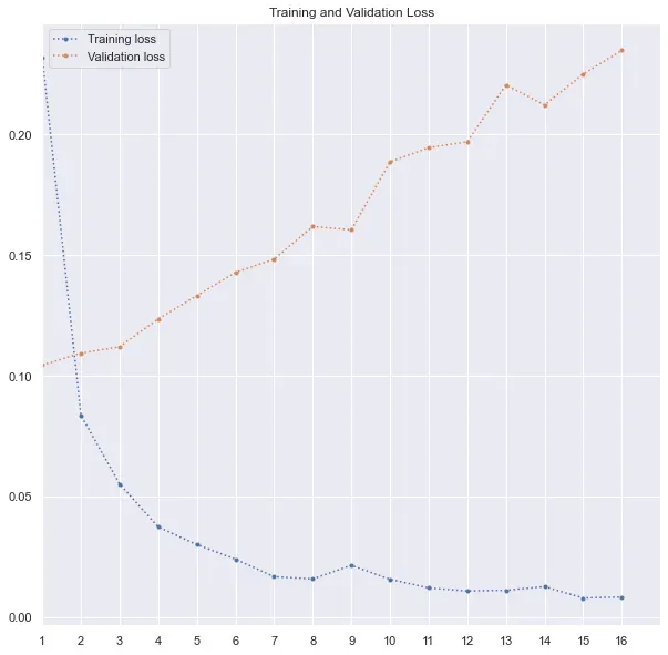
尽管可以对该模型进行潜在的改进，但该模型没有显着改进。它的准确率为 96.1%，f1 分数为 96.14%。

使用预训练的词嵌入——GloVe

现在，我们还可以使用预训练的词嵌入，比如 GloVe。 GloVe 是一种用于获取单词向量表示的无监督学习算法。对来自语料库的聚合全局词-词共现统计进行训练，得到的表示展示了词向量空间的有趣的线性子结构。 [4][0]

我使用的是用 60 亿个标记和 400k 词汇训练的那个，以 300 维向量格式表示。

在下面的代码中，我有一个代码可以在 Google Colab 上加载 GloVe，因为我部分地在 Colab 上工作。

# Load GloVe on Colab
!wget http://nlp.stanford.edu/data/glove.6B.zip
!unzip glove*.zip

f = open('/content/glove.6B.300d.txt')

for line in f:
    values = line.split()
    word = values[0]
    coefs = np.asarray(values[1:], dtype='float32')
    embeddings_index[word] = coefs
f.close()
print('Loaded {} word vectors.'.format(len(embeddings_index)))

在这里，我概述了如何从本地加载文件。从这里下载词嵌入。[0]

# Load local GloVe weights - Download the file and store it
embeddings_index = dict()
f = open('your/path/glove.6B/glove.6B.300d.txt', encoding='utf-8')
for line in f:
    values = line.split()
    word = values[0]
    coefs = np.asarray(values[1:], dtype='float32')
    embeddings_index[word] = coefs
f.close()
print('Loaded {} word vectors.'.format(len(embeddings_index)))

接下来，我们的目标是在 GloVe 嵌入中找到假新闻数据中的标记，并获得相应的权重。

# create a weight matrix for words in training docs
print('Get vocab_size')
vocab_size = len(tokenizer.word_index) + 1

print('Create the embedding matrix')
embedding_matrix = np.zeros((vocab_size, 300))
for word, i in tokenizer.word_index.items():
    embedding_vector = embeddings_index.get(word)
    if embedding_vector is not None:
        embedding_matrix[i] = embedding_vector

带手套的简单模型

现在，我已经为我们的训练数据嵌入了 GloVe，我使用了 output_dim=300 的 Embedding 层，这是 GloVe 矢量表示形状。另外，我使用了 trainable=False，因为我使用的是预训练的权重，所以我不应该在训练时更新它们。他们与其他词保持关系，所以最好不要打扰它。[0]

# The best model file name for uniformity
best_model_file_name = "models/best_model_simple_with_GloVe.hdf5"

# the model
def get_simple_GloVe_model():
    model = Sequential()
    model.add(Embedding(vocab_size, 
                        300, 
                        weights=[embedding_matrix], 
                        input_length=max_length,
                        trainable=False))
    model.add(Flatten())
    model.add(Dense(1, activation='sigmoid'))
    return model

callbacks=[
    keras.callbacks.EarlyStopping(monitor="val_loss", 
                                  patience=15, 
                                  verbose=1, 
                                  mode="min", 
                                  restore_best_weights=True),
    keras.callbacks.ModelCheckpoint(filepath=best_model_file_name, 
                                    verbose=1, 
                                    save_best_only=True)
]

model = get_simple_GloVe_model()
print(model.summary())

model.compile(loss='binary_crossentropy',
              optimizer='adam', 
              metrics=[tf.keras.metrics.Precision(), tf.keras.metrics.Recall()])

history = model.fit(X_train, 
                    y_train, 
                    epochs=50, 
                    validation_data=(X_test, y_test), 
                    callbacks=callbacks)

model = keras.models.load_model(best_model_file_name)
y_pred = (model.predict(X_test) > 0.5).astype("int32")
print('Accuracy: ', accuracy_score(y_test, y_pred))
print('Precision: ', precision_score(y_test, y_pred))
print('Recall: ', recall_score(y_test, y_pred))
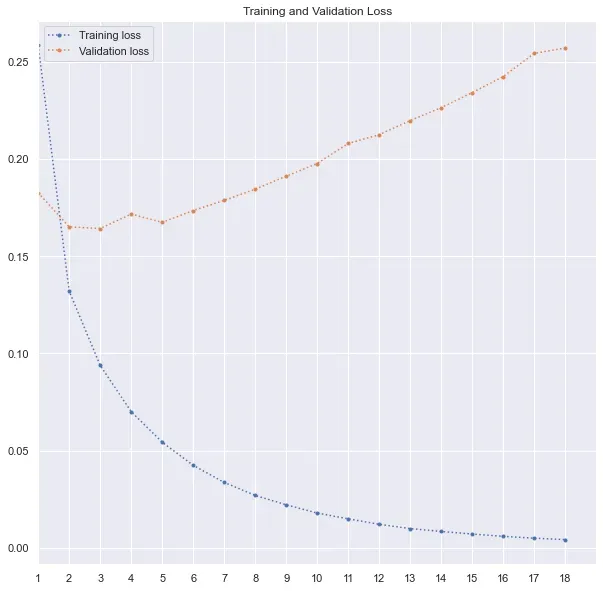
print('F1 Score: ', f1_score(y_test, y_pred))

最后，使用我之前使用的相同过程，我用 50 个 epoch 训练了模型。但是，由于在第 3 个 epoch 之后没有任何改善，因此模型在第 18 个 epoch 之后停止了训练。分数低于前两个模型。准确率和 f1 分数均为 ~93%。

GloVe with LSTM

而且..最后，我使用了 GloVe 嵌入来训练我之前使用的 LSTM 模型，以获得更好的结果。完整的代码如下 –

# The best model file name for uniformity
best_model_file_name = "models/best_model_LSTM_with_GloVe.hdf5"

# the model
def get_simple_GloVe_model():
    model = Sequential()
    model.add(Embedding(vocab_size, 
                        300, 
                        weights=[embedding_matrix], 
                        input_length=max_length,
                        trainable=False))
    model.add(LSTM(100))
    model.add(Dropout(0.3))
    model.add(Dense(64, activation='relu'))
    model.add(Dropout(0.3))
    model.add(Flatten())
    model.add(Dense(1, activation='sigmoid'))
    return model

callbacks=[
    keras.callbacks.EarlyStopping(monitor="val_loss", 
                                  patience=15, 
                                  verbose=1, 
                                  mode="min", 
                                  restore_best_weights=True),
    keras.callbacks.ModelCheckpoint(filepath=best_model_file_name, 
                                    verbose=1, 
                                    save_best_only=True)
]

model = get_simple_GloVe_model()
print(model.summary())

model.compile(loss='binary_crossentropy',
              optimizer='adam', 
              metrics=[tf.keras.metrics.Precision(), tf.keras.metrics.Recall()])

history = model.fit(X_train, 
                    y_train, 
                    epochs=50, 
                    validation_data=(X_test, y_test), 
                    callbacks=callbacks)

model = keras.models.load_model(best_model_file_name)
y_pred = (model.predict(X_test) > 0.5).astype("int32")
print('Accuracy: ', accuracy_score(y_test, y_pred))
print('Precision: ', precision_score(y_test, y_pred))
print('Recall: ', recall_score(y_test, y_pred))
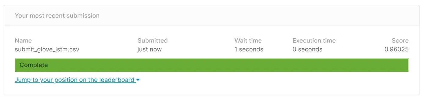
print('F1 Score: ', f1_score(y_test, y_pred))

同样，我使用了 50 个 epoch，并且在第三个 epoch 之后模型没有改善。因此，训练过程在第 18 个 epoch 之后停止。准确率和 f1 分数都提高到了 96.5%，接近第一个 Keras 模型。

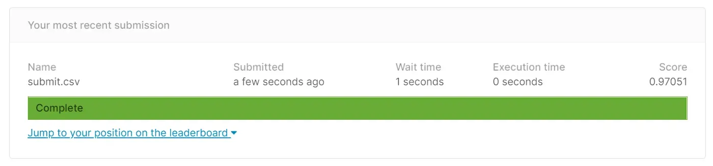
所以，我在 Kaggle 的测试数据上尝试了这个模型的预测，这是我的结果——

Conclusion

在本练习中，最佳模型是调整后的 Logistic 回归模型。这个用例有很多需要进一步改进的空间，尤其是设计更好的深度学习模型。此外，出于时间考虑，我没有调整 Random Forest 和 AdaBoost 分类器，这可能会比 Logistic 回归带来更好的性能。

References

1. https://faroit.com/keras-docs/1.0.1/getting-started/sequential-model-guide/[0]
2. https://colah.github.io/posts/2015-08-Understanding-LSTMs/[0]
3. https://machinelearningmastery.com/use-word-embedding-layers-deep-learning-keras/[0]
4. https://nlp.stanford.edu/projects/glove/[0]

完整的代码在这里。[0]

Thanks for visiting!

我的链接：中 |领英 | GitHub[0][1][2]