2022-ConvNet CVPR
论文地址:https://arxiv.org/abs/2201.03545
代码地址: https://github.com/facebookresearch/ConvNeXt
感谢我的研究生导师!!!
1. 简介
1.1 简介
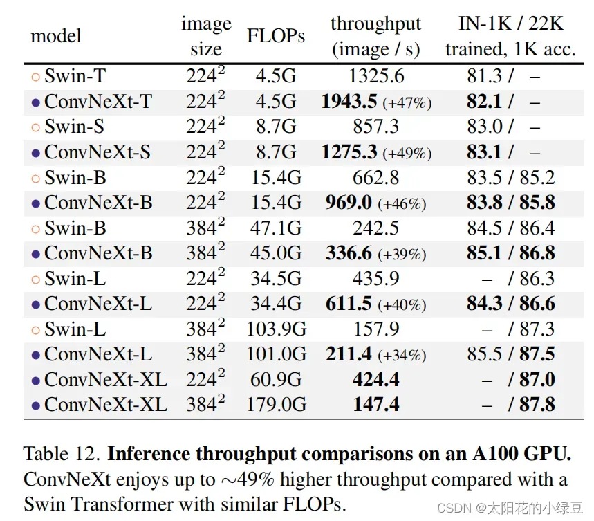
今年(2022)一月份,Facebook AI Research和UC Berkeley一起发表了一篇文章A ConvNet for the 2020s,在文章中提出了ConvNeXt纯卷积神经网络,它对标的是2021年非常火的Swin Transformer,通过一系列实验比对,在相同的FLOPs下,ConvNeXt相比Swin Transformer拥有更快的推理速度以及更高的准确率,在ImageNet 22K上ConvNeXt-XL达到了87.8%的准确率。看来ConvNeXt的提出强行给卷积神经网络续了口命。
1.2 结论
自从ViT(Vision Transformer)在CV领域大放异彩,越来越多的研究人员开始拥入Transformer的怀抱。
回顾近一年,在CV领域发的文章绝大多数都是基于Transformer的,比如2021年ICCV 的best paper Swin Transformer
而卷积神经网络已经开始慢慢淡出舞台中央。卷积神经网络要被Transformer取代了吗?也许会在不久的将来。
今年(2022)一月份,Facebook AI Research和UC Berkeley一起发表了一篇文章A ConvNet for the 2020s,在文章中提出了ConvNeXt纯卷积神经网络,它对标的是2021年非常火的Swin Transformer,通过一系列实验比对,在相同的FLOPs下,ConvNeXt相比Swin Transformer拥有更快的推理速度以及更高的准确率,在ImageNet 22K上ConvNeXt-XL达到了87.8%的准确率,参看下图(原文表12)。看来ConvNeXt的提出强行给卷积神经网络续了口命。
2. 网络架构
如果你仔细阅读了这篇文章,你会发现ConvNeXt“毫无亮点”,ConvNeXt使用的全部都是现有的结构和方法,没有任何结构或者方法的创新。而且源码也非常的精简,100多行代码就能搭建完成,相比Swin Transformer简直不要太简单。
2.1 设计方案
如果你仔细阅读了这篇文章,你会发现ConvNeXt“毫无亮点”,ConvNeXt使用的全部都是现有的结构和方法,没有任何结构或者方法的创新。而且源码也非常的精简,100多行代码就能搭建完成,相比Swin Transformer简直不要太简单。
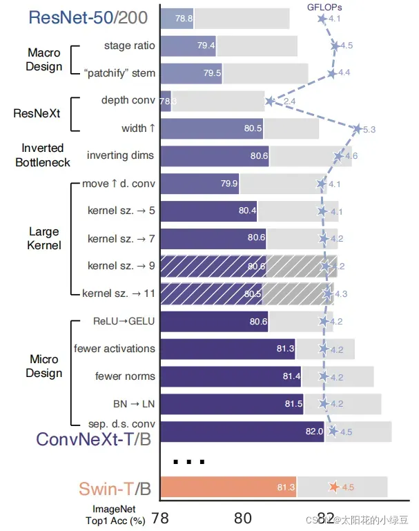
- macro design
- ResNeXt
- inverted bottleneck
- large kerner size
- various layer-wise micro designs
下图(原论文图2)展现了每个方案对最终结果的影响(Imagenet 1K的准确率)。很明显最后得到的ConvNeXt在相同FLOPs下准确率已经超过了Swin Transformer。接下来,针对每一个实验进行解析。
2.2 Macro design
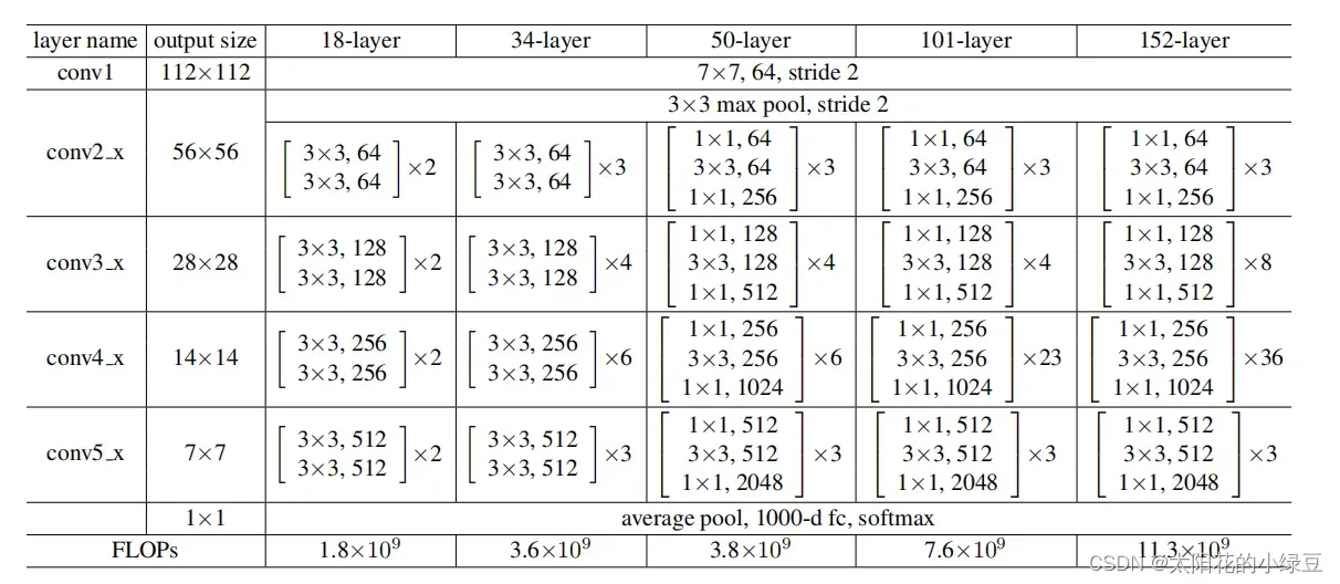
在原ResNet网络中,一般conv4_x(即stage3)堆叠的block的次数是最多的。如下图中的ResNet50中stage1到stage4堆叠block的次数是(3, 4, 6, 3)比例大概是1:1:2:1,但在Swin Transformer中,比如Swin-T的比例是1:1:3:1,Swin-L的比例是1:1:9:1。很明显,在Swin Transformer中,stage3堆叠block的占比更高。所以作者就将ResNet50中的堆叠次数由(3, 4, 6, 3)调整成(3, 3, 9, 3),和Swin-T拥有相似的FLOPs。进行调整后,准确率由78.8%提升到了79.4%。
在之前的卷积神经网络中,一般最初的下采样模块stem一般都是通过一个卷积核大小为7x7步距为2的卷积层以及一个步距为2的最大池化下采样共同组成,高和宽都下采样4倍。但在Transformer模型中一般都是通过一个卷积核非常大且相邻窗口之间没有重叠的(即stride等于kernel_size)卷积层进行下采样。比如在Swin Transformer中采用的是一个卷积核大小为4x4步距为4的卷积层构成patchify,同样是下采样4倍。所以作者将ResNet中的stem也换成了和Swin Transformer一样的patchify。替换后准确率从79.4% 提升到79.5%,并且FLOPs也降低了一点。
2.3 ResNeXt-ify
接下来作者借鉴了ResNeXt中的组卷积grouped convolution,因为ResNeXt相比普通的ResNet而言在FLOPs以及accuracy之间做到了更好的平衡。而作者采用的是更激进的depthwise convolution,即group数和通道数channel相同,这样做的另一个原因是作者认为depthwise convolution和self-attention中的加权求和操作很相似。
接着作者将最初的通道数由64调整成96和Swin Transformer保持一致,最终准确率达到了80.5%。
2.4 Inverted Bottleneck
作者认为Transformer block中的MLP模块非常像MobileNetV2中的Inverted Bottleneck模块,即两头细中间粗。
图a是ReNet中采用的Bottleneck模块,
b是MobileNetV2采用的Inverted Botleneck模块
c是ConvNeXt采用的是Inverted Bottleneck模块。
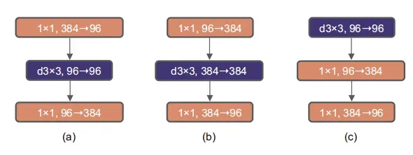
作者采用Inverted Bottleneck模块后,在较小的模型上准确率由80.5%提升到了80.6%,在较大的模型上准确率由81.9%提升到82.6%。
2.5 Large Kernel Sizes
在Transformer中一般都是对全局做self-attention,比如Vision Transformer。即使是Swin Transformer也有7x7大小的窗口。但现在主流的卷积神经网络都是采用3x3大小的窗口,因为之前VGG论文中说通过堆叠多个3x3的窗口可以替代一个更大的窗口,而且现在的GPU设备针对3x3大小的卷积核做了很多的优化,所以会更高效。接着作者做了如下两个改动:
- Moving up depthwise conv layer**,即将
depthwise conv模块上移,原来是1x1 conv->depthwise conv->1x1 conv,现在变成了depthwise conv->1x1 conv->1x1 conv。这么做是因为在Transformer中,MSA模块是放在MLP模块之前的,所以这里进行效仿,将depthwise conv上移。这样改动后,准确率下降到了79.9%,同时FLOPs也减小了。
Increasing the kernel size,接着作者将depthwise conv的卷积核大小由3x3改成了7x7(和Swin Transformer一样),当然作者也尝试了其他尺寸,包括3, 5, 7, 9, 11发现取到7时准确率就达到了饱和。并且准确率从79.9% (3×3) 增长到 80.6% (7×7)。
2.6 Micro Design
接下来作者在聚焦到一些更细小的差异,比如激活函数以及Normalization。
Replacing ReLU with GELU,在Transformer中激活函数基本用的都是GELU,而在卷积神经网络中最常用的是ReLU,于是作者又将激活函数替换成了GELU,替换后发现准确率没变化。
Fewer activation functions,使用更少的激活函数。在卷积神经网络中,一般会在每个卷积层或全连接后都接上一个激活函数。但在Transformer中并不是每个模块后都跟有激活函数,比如MLP中只有第一个全连接层后跟了GELU激活函数。接着作者在ConvNeXt Block中也减少激活函数的使用,如下图所示,减少后发现准确率从80.6%增长到81.3%。
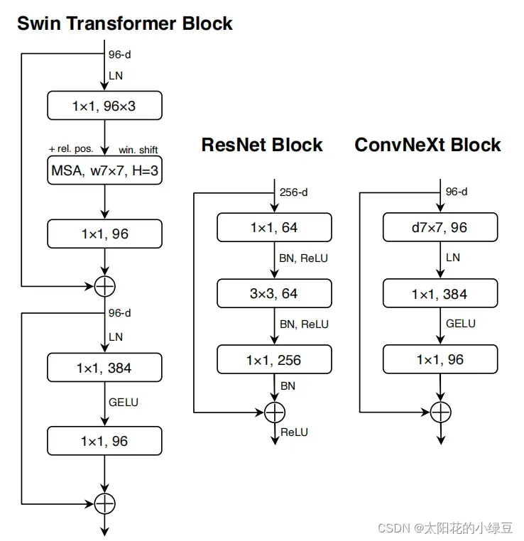
- Fewer normalization layers,使用更少的Normalization。同样在
Transformer中,Normalization使用的也比较少,接着作者也减少了ConvNeXt Block中的Normalization层,只保留了depthwise conv后的Normalization层。此时准确率已经达到了81.4%,已经超过了Swin-T。 - Substituting BN with LN,将BN替换成LN。Batch Normalization(BN)在卷积神经网络中是非常常用的操作了,它可以加速网络的收敛并减少过拟合(但用的不好也是个大坑)。但在
Transformer中基本都用的Layer Normalization(LN),因为最开始Transformer是应用在NLP领域的,BN又不适用于NLP相关任务。接着作者将BN全部替换成了LN,发现准确率还有小幅提升达到了81.5%。 - Separate downsampling layers,单独的下采样层。在
ResNet网络中stage2-stage4的下采样都是通过将主分支上3x3的卷积层步距设置成2,捷径分支上1x1的卷积层步距设置成2进行下采样的。但在Swin Transformer中是通过一个单独的Patch Merging实现的。接着作者就为ConvNext网络单独使用了一个下采样层,就是通过一个Laryer Normalization加上一个卷积核大小为2步距为2的卷积层构成。更改后准确率就提升到了82.0%。
2.7 ConvNext variants
对于ConvNeXt网络,作者提出了T/S/B/L四个版本,计算复杂度刚好和Swin Transformer中的T/S/B/L相似。
- ConvNeXt-T: C = (96, 192, 384, 768), B = (3, 3, 9, 3)
- ConvNeXt-S: C = (96, 192, 384, 768), B = (3, 3, 27, 3)
- ConvNeXt-B: C = (128, 256, 512, 1024), B = (3, 3, 27, 3)
- ConvNeXt-L: C = (192, 384, 768, 1536), B = (3, 3, 27, 3)
- ConvNeXt-XL: C = (256, 512, 1024, 2048), B = (3, 3, 27, 3)
其中C代表4个stage中输入的通道数,B代表每个stage重复堆叠block的次数。
3. 训练
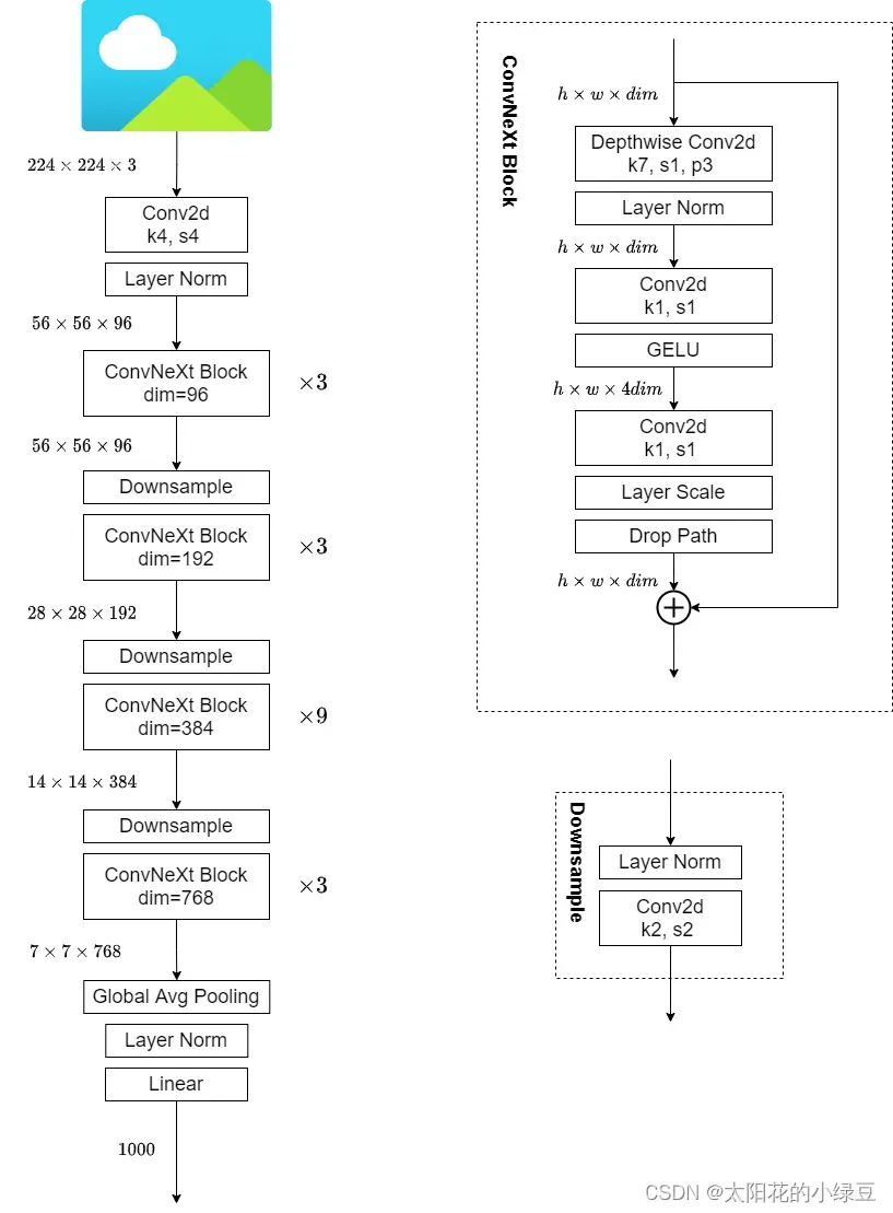
下图是我根据源码手绘的ConvNeXt-T网络结构图,仔细观察ConvNeXt Block会发现其中还有一个Layer Scale操作
(论文中并没有提到),其实它就是将输入的特征层乘上一个可训练的参数,该参数就是一个向量
元素个数与特征层channel相同,即对每个channel的数据进行缩放。
Layer Scale操作出自于Going deeper with image transformers. ICCV, 2021这篇文章
4. 代码
import torch
import torch.nn as nn
import torch.nn.functional as F
from torchvision.models import resnext50_32x4d

def drop_path(x, drop_prob: float = 0., training: bool = False):
    """Drop paths (Stochastic Depth) per sample (when applied in main path of residual blocks).
    This is the same as the DropConnect impl I created for EfficientNet, etc networks, however,
    the original name is misleading as 'Drop Connect' is a different form of dropout in a separate paper...
    See discussion: https://github.com/tensorflow/tpu/issues/494#issuecomment-532968956 ... I've opted for
    changing the layer and argument names to 'drop path' rather than mix DropConnect as a layer name and use
    'survival rate' as the argument.
    """
    if drop_prob == 0. or not training:
        return x
    keep_prob = 1 - drop_prob
    shape = (x.shape[0],) + (1,) * (x.ndim - 1)  # work with diff dim tensors, not just 2D ConvNets
    random_tensor = keep_prob + torch.rand(shape, dtype=x.dtype, device=x.device)
    random_tensor.floor_()  # binarize
    output = x.div(keep_prob) * random_tensor
    return output


class DropPath(nn.Module):
    """Drop paths (Stochastic Depth) per sample  (when applied in main path of residual blocks).
    """

    def __init__(self, drop_prob=None):
        super(DropPath, self).__init__()
        self.drop_prob = drop_prob

    def forward(self, x):
        return drop_path(x, self.drop_prob, self.training)


class LayerNorm(nn.Module):
    r""" LayerNorm that supports two data formats: channels_last (default) or channels_first.
    The ordering of the dimensions in the inputs. channels_last corresponds to inputs with
    shape (batch_size, height, width, channels) while channels_first corresponds to inputs
    with shape (batch_size, channels, height, width).
    """

    def __init__(self, normalized_shape, eps=1e-6, data_format="channels_last"):
        super().__init__()
        self.weight = nn.Parameter(torch.ones(normalized_shape), requires_grad=True)
        self.bias = nn.Parameter(torch.zeros(normalized_shape), requires_grad=True)
        self.eps = eps
        self.data_format = data_format
        if self.data_format not in ["channels_last", "channels_first"]:
            raise ValueError(f"not support data format '{self.data_format}'")
        self.normalized_shape = (normalized_shape,)

    def forward(self, x: torch.Tensor) -> torch.Tensor:
        if self.data_format == "channels_last":
            return F.layer_norm(x, self.normalized_shape, self.weight, self.bias, self.eps)
        elif self.data_format == "channels_first":
            # [batch_size, channels, height, width]
            mean = x.mean(1, keepdim=True)
            var = (x - mean).pow(2).mean(1, keepdim=True)
            x = (x - mean) / torch.sqrt(var + self.eps)
            x = self.weight[:, None, None] * x + self.bias[:, None, None]
            return x


class Block(nn.Module):
    r""" ConvNeXt Block. There are two equivalent implementations:
    (1) DwConv -> LayerNorm (channels_first) -> 1x1 Conv -> GELU -> 1x1 Conv; all in (N, C, H, W)
    (2) DwConv -> Permute to (N, H, W, C); LayerNorm (channels_last) -> Linear -> GELU -> Linear; Permute back
    We use (2) as we find it slightly faster in PyTorch
    Args:
        dim (int): Number of input channels.
        drop_rate (float): Stochastic depth rate. Default: 0.0
        layer_scale_init_value (float): Init value for Layer Scale. Default: 1e-6.
    """

    def __init__(self, dim, drop_rate=0., layer_scale_init_value=1e-6):
        super().__init__()
        self.dwconv = nn.Conv2d(dim, dim, kernel_size=7, padding=3, groups=dim)  # depthwise conv
        self.norm = LayerNorm(dim, eps=1e-6, data_format="channels_last")
        self.pwconv1 = nn.Linear(dim, 4 * dim)  # pointwise/1x1 convs, implemented with linear layers
        self.act = nn.GELU()
        self.pwconv2 = nn.Linear(4 * dim, dim)
        self.gamma = nn.Parameter(layer_scale_init_value * torch.ones((dim,)),
                                  requires_grad=True) if layer_scale_init_value > 0 else None
        self.drop_path = DropPath(drop_rate) if drop_rate > 0. else nn.Identity()

    def forward(self, x: torch.Tensor) -> torch.Tensor:
        shortcut = x
        x = self.dwconv(x)
        x = x.permute(0, 2, 3, 1)  # [N, C, H, W] -> [N, H, W, C]
        x = self.norm(x)
        x = self.pwconv1(x)
        x = self.act(x)
        x = self.pwconv2(x)
        if self.gamma is not None:
            x = self.gamma * x
        x = x.permute(0, 3, 1, 2)  # [N, H, W, C] -> [N, C, H, W]

        x = shortcut + self.drop_path(x)
        return x


class ConvNeXt(nn.Module):
    r""" ConvNeXt
        A PyTorch impl of : `A ConvNet for the 2020s`  -
          https://arxiv.org/pdf/2201.03545.pdf
    Args:
        in_chans (int): Number of input image channels. Default: 3
        num_classes (int): Number of classes for classification head. Default: 1000
        depths (tuple(int)): Number of blocks at each stage. Default: [3, 3, 9, 3]
        dims (int): Feature dimension at each stage. Default: [96, 192, 384, 768]
        drop_path_rate (float): Stochastic depth rate. Default: 0.
        layer_scale_init_value (float): Init value for Layer Scale. Default: 1e-6.
        head_init_scale (float): Init scaling value for classifier weights and biases. Default: 1.
    """

    def __init__(self, in_chans: int = 3, num_classes: int = 1000, depths: list = None,
                 dims: list = None, drop_path_rate: float = 0., layer_scale_init_value: float = 1e-6,
                 head_init_scale: float = 1.):
        super().__init__()
        self.downsample_layers = nn.ModuleList()  # stem and 3 intermediate downsampling conv layers
        stem = nn.Sequential(nn.Conv2d(in_chans, dims[0], kernel_size=4, stride=4),
                             LayerNorm(dims[0], eps=1e-6, data_format="channels_first"))
        self.downsample_layers.append(stem)

        # 对应stage2-stage4前的3个downsample
        for i in range(3):
            downsample_layer = nn.Sequential(LayerNorm(dims[i], eps=1e-6, data_format="channels_first"),
                                             nn.Conv2d(dims[i], dims[i + 1], kernel_size=2, stride=2))
            self.downsample_layers.append(downsample_layer)

        self.stages = nn.ModuleList()  # 4 feature resolution stages, each consisting of multiple blocks
        dp_rates = [x.item() for x in torch.linspace(0, drop_path_rate, sum(depths))]
        cur = 0
        # 构建每个stage中堆叠的block
        for i in range(4):
            stage = nn.Sequential(
                *[Block(dim=dims[i], drop_rate=dp_rates[cur + j], layer_scale_init_value=layer_scale_init_value)
                  for j in range(depths[i])]
            )
            self.stages.append(stage)
            cur += depths[i]

        self.norm = nn.LayerNorm(dims[-1], eps=1e-6)  # final norm layer
        self.head = nn.Linear(dims[-1], num_classes)
        self.apply(self._init_weights)
        self.head.weight.data.mul_(head_init_scale)
        self.head.bias.data.mul_(head_init_scale)

    def _init_weights(self, m):
        if isinstance(m, (nn.Conv2d, nn.Linear)):
            nn.init.trunc_normal_(m.weight, std=0.2)
            nn.init.constant_(m.bias, 0)

    def forward_features(self, x: torch.Tensor) -> torch.Tensor:
        for i in range(4):
            x = self.downsample_layers[i](x)
            x = self.stages[i](x)

        return self.norm(x.mean([-2, -1]))  # global average pooling, (N, C, H, W) -> (N, C)

    def forward(self, x: torch.Tensor) -> torch.Tensor:
        x = self.forward_features(x)
        x = self.head(x)
        return x


def convnext_tiny(num_classes: int):
    # https://dl.fbaipublicfiles.com/convnext/convnext_tiny_1k_224_ema.pth
    model = ConvNeXt(depths=[3, 3, 9, 3],
                     dims=[96, 192, 384, 768],
                     num_classes=num_classes,
                     drop_path_rate=0.2)
    return model


def convnext_small(num_classes: int):
    # https://dl.fbaipublicfiles.com/convnext/convnext_small_1k_224_ema.pth
    model = ConvNeXt(depths=[3, 3, 27, 3],
                     dims=[96, 192, 384, 768],
                     num_classes=num_classes)
    return model


def convnext_base(num_classes: int):
    # https://dl.fbaipublicfiles.com/convnext/convnext_base_1k_224_ema.pth
    # https://dl.fbaipublicfiles.com/convnext/convnext_base_22k_224.pth
    model = ConvNeXt(depths=[3, 3, 27, 3],
                     dims=[128, 256, 512, 1024],
                     num_classes=num_classes)
    return model


def convnext_large(num_classes: int):
    # https://dl.fbaipublicfiles.com/convnext/convnext_large_1k_224_ema.pth
    # https://dl.fbaipublicfiles.com/convnext/convnext_large_22k_224.pth
    model = ConvNeXt(depths=[3, 3, 27, 3],
                     dims=[192, 384, 768, 1536],
                     num_classes=num_classes)
    return model


def convnext_xlarge(num_classes: int):
    # https://dl.fbaipublicfiles.com/convnext/convnext_xlarge_22k_224.pth
    model = ConvNeXt(depths=[3, 3, 27, 3],
                     dims=[256, 512, 1024, 2048],
                     num_classes=num_classes)
    return model


if __name__ == '__main__':
    # from torchsummary import summary
    #
    # device = torch.device('cuda' if torch.cuda.is_available() else 'cpu')
    # model = convnext_tiny(num_classes=5)
    # model.to(device)
    # print(model)
    # x = torch.randn(1,3,224,224,device=device)
    # y = model(x)
    # print(y)

    # summary(model, input_size=(3, 224, 224))
    from thop import profile
    model = convnext_tiny(num_classes=5)
    input = torch.randn(1, 3, 224, 224)
    flops, params = profile(model, inputs=(input,))
    print("flops:{:.3f}G".format(flops/1e9))
    print("params:{:.3f}M".format(params/1e6))
参考资料
文章出处登录后可见!