同步压缩变换原理
作为处理非平稳信号的有力工具,时频分析在时域和频域联合表征信号,是时间和频率的二元函数。传统的时频分析工具主要分为线性方法和二次方法。线性方法受到海森堡测不准原理的制约,二次方法存在交叉项的干扰。
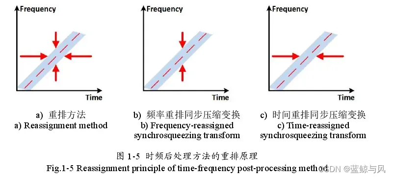
为了提升时频聚集性,逼近理想的时频表示,时频重排 (Reassignment method, RM)作为一种后处理技术被提。它在二维的时频面上重排时频系数,导致其丧失了重构信号的能力。同步压缩变换作为一种特殊的重排,不仅可以锐化时频表示,还能恢复信号。因此,同步压缩变换受到研究学者的热爱。
同步压缩变换主要有两种框架,一种基于小波变换,另一种基于短时傅里叶变换。本文中以小波变换为框架,介绍同步压缩变换。在2011年,Daubechies等人提出了同步压缩小波变换,作为一种经验模态分解工具。它的主要思想是将小波变换的系数重新分配到估计的瞬时频率处。所以,同步压缩变换的核心是估计瞬时频率。通常,是对时频表示关于时间求导,估计信号的瞬时频率。然后,把系数挤压到估计的瞬时频率处。尽管,同步压缩小波变换有很多改进形式。但是,万变不离其宗,都是同样的套路。重排和同步压缩变换的主要思想如下,
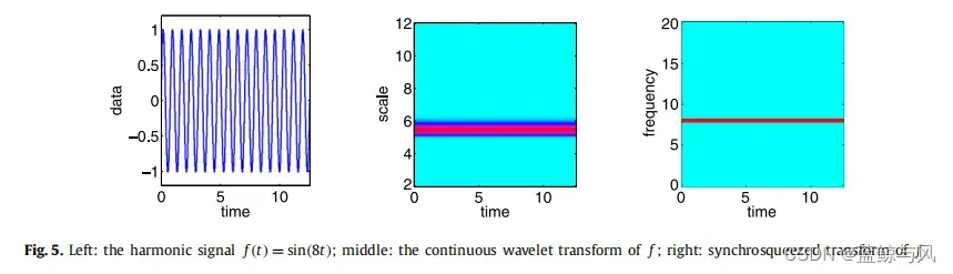
下图是2011年论文中,一个谐波信号的小波变换和同步压缩小波变换的结果对比。左边是谐波信号的时域波形,中间是小波变换,右边是同步压缩小波变换的结果。显然,小波变换的系数分布在瞬时频率8Hz的周围,同步压缩小波变换的系数就只分布在8Hz处。换句话说,同步压缩小波变换的时频分辨率更高,能量聚集性更高。一般通过瑞利熵来衡量时频表示的能量聚集性,但是对于真实信号这并不是合理的选择。
同步压缩小波变换代码
主程序
clear ;
close all ;
clc;


%% fix the seed
initstate(23400) ;
opts = struct();
opts.motherwavelet = 'morlet' ;%morlet,Cinfc
opts.CENTER = 1;
opts.FWHM = 0.2;


fs=2^9;    %采样频率
dt=1/fs;    %时间精度
timestart=0;
timeend=1;
t=(0:(timeend-timestart)/dt-1)*dt+timestart;
t=t';
k1=35;
f1=60;
y=exp((1i)*pi*k1*t.*t+2*pi*1i*f1*t).*(t>=0& t<timeend);


freqlow=0;
freqhigh=128;
alpha=1;
seta=-acot(k1);
f=freqlow:alpha:freqhigh;
e=t(end);


%注意SQCWT中列为尺度,行为时间
[tfr, tfrsq, tfrtic, tfrsqtic] = sqCWT(t, y, freqlow, freqhigh, alpha, opts);

figure();
imagesc(t,tfrtic,abs(tfr));
set(gca,'ydir','normal');
xlabel('Time(s)','FontSize',12,'FontName','Times New Roman');
ylabel('Scales','FontSize',12,'FontName','Times New Roman');
set(gca,'FontSize',16,'FontName','Times New Roman')
set(gca,'linewidth',1);


%
figure()
imagesc(t,f, abs(tfrsq));
set(gca,'ydir','normal');
xlabel('Time(s)','FontSize',12,'FontName','Times New Roman');
ylabel('Frequency(Hz)','FontSize',12,'FontName','Times New Roman');
set(gca,'FontSize',16,'FontName','Times New Roman')
set(gca,'linewidth',1);
同步压缩变换核心代码
function [tfr, tfrsq, tfrtic, tfrsqtic] = sqCWT(t, x, freqlow, freqhigh, alpha, opts);

%
% Synchrosqueezing transform ver 0.5 (2015-03-09)
% You can find more information in
%	http://sites.google.com/site/hautiengwu/
%
% Example: [~, tfrsq, ~, tfrsqtic] = sqCWT(time, xm, lowfreq, highfreq, alpha, opts);
%	time: 	time of the signal
%	xm: 	the signal to be analyzed
%	[lowfreq, highfreq]: the frequency range in the output time-frequency representation. For the sake of computational efficiency.
%	alpha:	the frequency resolution in the output time-frequency representation
%	opts:	parameters for the CWT analysis. See below
%	tfr/tfrtic:	the CWT and its scale tic
%	tfrsq/tfrsqtic: the SST-CWT and its frequency tic
%
% by Hau-tieng Wu v0.1 2011-06-20 (hauwu@math.princeton.edu)
%		  v0.2 2011-09-10
%		  v0.3 2012-03-03
%		  v0.4 2012-12-12
%		  v0.5 2015-03-09

	%% you can play with these 4 parameters, but the results might not be
	%% that different if the change is not crazy
Gamma = 1e-8;
nvoice = 32;
scale = 2;
oct = 1;

%++++++++++++++++++++++++++++++++++++++++++++++++++++++++++++++++++++++++++
noctave = floor(log2(length(x))) - oct;
dt = t(2) - t(1);


%+++++++++++++++++++++++++++++++++++++++++++++++++++++++++++++++++++++++++++
    %% Continuous wavelet transform

[tfr, tfrtic] = CWT(t, x, oct, scale, nvoice, opts) ;
% tfr=tfr';
% tfrtic=tfrtic';
%行时间,列尺度
Dtfr = (-i/2/pi/dt)*[tfr(2:end,:) - tfr(1:end-1,:); tfr(end,:)-tfr(end-1,:)] ;
% Dtfr=(-1i/2/pi/dt)*[tfr(:,2:end)-tfr(:,1:end-1) tfr(:,end)-tfr(:,end-1)] /(dt);
Dtfr((abs(tfr) < Gamma)) = NaN;
omega = Dtfr./tfr;

%+++++++++++++++++++++++++++++++++++++++++++++++++++++++++++++++++++++++++++++
    	%% Synchro-squeezing transform

[tfrsq, tfrsqtic] = SQ(tfr, omega, alpha, scale, nvoice, freqlow, freqhigh);
tfr = transpose(tfr) ;
tfrsq = transpose(tfrsq) ;

end


%=====================================================================
	%% function for CWT-based SST
function [tfrsq, freq] = SQ(tfd, omega, alpha, scale, nvoice, freqlow, freqhigh);
omega = abs(omega);
[n, nscale] = size(tfd);

nalpha = floor((freqhigh - freqlow)./alpha);
tfrsq = zeros(n, nalpha);
freq = ([1:1:nalpha])*alpha + freqlow;
nfreq = length(freq);

for b = 1:n             %% Synchro-
    for kscale = 1: nscale       %% -Squeezing

%         qscale = scale .* (2^(kscale/nvoice));
        qscale = scale .* (2^(kscale/nvoice));

        if (isfinite(omega(b, kscale)) && (omega(b, kscale)>0))
            k = floor( ( omega(b,kscale) - freqlow )./ alpha )+1;

            if (isfinite(k) && (k > 0) && (k < nfreq-1))
	        ha = freq(k+1)-freq(k);
                tfrsq(b,k) = tfrsq(b,k) + log(2)*tfd(b,kscale)*sqrt(qscale)./ha/nvoice;
            end
        end
    end
end
end
小波变换代码
function [tfr, tfrtic] = newOmega(t, x, oct, scale, nvoice, opts)
%
% Continuous wavelet transform ver 0.1
% Modified from wavelab 85
%
% INPUT:
% OUTPUT:
% DEPENDENCY:
%
% by Hau-tieng Wu 2011-06-20 (hauwu@math.princeton.edu)
% by Hau-tieng Wu 2012-12-23 (hauwu@math.princeton.edu)
%

%++++++++++++++++++++++++++++++++++++++++++++++++++++++++++++++++++++++++++
%% prepare for the input

if nargin < 6
    opts = struct();
    opts.motherwavelet = 'Cinfc' ;
    opts.CENTER = 1 ;
    opts.FWHM = 0.3 ;
end

if nargin < 5
    nvoice = 32;
end

if nargin < 4
    scale = 2;
end

if nargin < 3
    oct = 1;
end


%++++++++++++++++++++++++++++++++++++++++++++++++++++++++++++++++++++++++++
    %% start to do CWT

dt = t(2)-t(1);
n = length(x);
    %% assume the original signal is on [0,L].
    %% assume the signal is on [0,1]. Frequencies are rescaled to \xi/L
xi = [(0:(n/2)) (((-n/2)+1):-1)]; xi = xi(:);
xhat = fft(x);

noctave = floor(log2(n)) - oct;
tfr = zeros(n, nvoice .* noctave);
kscale = 1;

tfrtic = zeros(1, nvoice .* noctave);
for jj = 1 : nvoice .* noctave
    tfrtic(jj) = scale .* (2^(jj/nvoice));
end

for jo = 1:noctave	% # of scales
    for jv = 1:nvoice

    	qscale = scale .* (2^(jv/nvoice));
    	omega =  xi ./ qscale ;

        if strcmp(opts.motherwavelet, 'morse');

			error('To use Morse wavelet, you have to download it...') ;

        elseif strcmp(opts.motherwavelet, 'Cinfc');

            tmp0 = (omega-opts.CENTER)./opts.FWHM;
            tmp1 = (tmp0).^2-1;

            windowq = exp( 1./tmp1 );
            windowq( find( omega >= (opts.CENTER+opts.FWHM) ) ) = 0;
            windowq( find( omega <= (opts.CENTER-opts.FWHM) ) ) = 0;

        elseif strcmp(opts.motherwavelet, 'morlet')

            windowq = 4*sqrt(pi)*exp(-4*(omega-0.69*pi).^2)-4.89098d-4*4*sqrt(pi)*exp(-4*omega.^2);

        elseif strcmp(opts.motherwavelet, 'gaussian');

            psihat = @(f) exp( -log(2)*( 2*(f-opts.CENTER)./opts.FWHM ).^2 );
            windowq = psihat(omega);


        elseif strcmp(opts.motherwavelet, 'meyer');  %% Meyer

            windowq = zeros(size(omega));
            int1 = find((omega>=5./8*0.69*pi)&(omega<0.69*pi));
            int2 = find((omega>=0.69*pi)&(omega<7./4*0.69*pi));
            windowq(int1) = sin(pi/2*meyeraux((omega(int1)-5./8*0.69*pi)/(3./8*0.69*pi)));
            windowq(int2) = cos(pi/2*meyeraux((omega(int2)-0.69*pi)/(3./4*0.69*pi)));

        elseif strcmp(opts.motherwavelet, 'BL3');    %% B-L 3

            phihat = (2*pi)^(-0.5)*(sin(omega/4)./(omega/4)).^4; phihat(1) = (2*pi)^(-0.5);
            aux1 = 151./315 + 397./840*cos(omega/2) + 1./21*cos(omega) + 1./2520*cos(3*omega/2);
            phisharphat = phihat.*(aux1.^(-0.5));

            aux2 = 151./315 - 397./840*cos(omega/2) + 1./21*cos(omega) - 1./2520*cos(3*omega/2);
            aux3 = 151./315 + 397./840*cos(omega) + 1./21*cos(2*omega) + 1./2520*cos(3*omega);
            msharphat = sin(omega/4).^4.*(aux2.^(0.5)).*(aux3.^(-0.5));
            windowq = phisharphat.*msharphat.*exp(i*omega/2).*(omega>=0);

	end

        windowq = windowq ./ sqrt(qscale);

        what = windowq .* xhat;

        w = ifft(what);
        tfr(:,kscale) = transpose(w);
        kscale = kscale+1;

    end

    scale = scale .* 2;

end


%++++++++++++++++++++++++++++++++++++++++++++++++++++++++++++++++++++++++
    %% calculate the constant for reconstruction
    %% TODO: calculate Rpsi for other mother wavelets
xi = [0.05:1/10000:10];

if strcmp(opts.motherwavelet, 'gaussian');   %% Gaussian (not really wavelet)

    psihat = @(f) exp( -log(2)*( 2*(f-opts.CENTER)./opts.FWHM ).^2 );
    windowq = psihat(xi);
    Rpsi = sum(windowq./xi)/10000;


elseif strcmp(opts.motherwavelet, 'morlet');

    windowq = 4*sqrt(pi)*exp(-4*(xi-0.69*pi).^2)-4.89098d-4*4*sqrt(pi)*exp(-4*xi.^2);
    Rpsi = sum(windowq./xi)/10000;

elseif strcmp(opts.motherwavelet, 'Cinfc');

    tmp0 = (xi - opts.CENTER)./opts.FWHM;
    tmp1 = (tmp0).^2-1;

    windowq = exp( 1./tmp1 );
    windowq( find( xi >= (opts.CENTER+opts.FWHM) ) ) = 0;
    windowq( find( xi <= (opts.CENTER-opts.FWHM) ) ) = 0;
    Rpsi = sum(windowq./xi)/10000;

else

	fprintf('Normalization is not implemented for Other mother wavelets, like BL3 and Meyer\n') ;

end


tfr = tfr ./ Rpsi;


end
实验结果
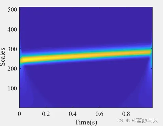
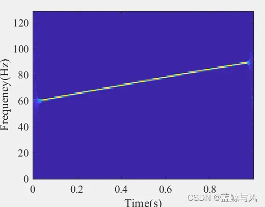
第一个为小波结果,第二个为同步压缩小波变换结果。同步压缩小波变换将小波系数挤压到瞬时频率处,所以它具有更加聚集的能量。小波变换的瑞利熵结果为13.1316,同步压缩小波变换的瑞利熵结果为8.8856。
[1] 何周杰. 同步变换理论、方法及其在工程信号分析中的应用[D].上海交通大学, 2020.
[2] ] I. Daubechies, J. Lu, H.-T. Wu, Synchrosqueezed wavelet transforms: an empirical mode decomposition-like tool, Appl. Comput. Harmon. Anal. 30 (2) (2011)243–261.
文章出处登录后可见!