AIGC专栏9——Scalable Diffusion Models with Transformers （DiT）结构解析

AIGC专栏9——Scalable Diffusion Models with Transformers （DiT）结构解析

• 学习前言
• 源码下载地址
• 网络构建
• • 一、什么是Diffusion Transformer (DiT)
  • 二、DiT的组成
  • 三、生成流程
  • • 1、采样流程
    • • a、生成初始噪声
      • b、对噪声进行N次采样
      • c、单次采样解析
      • • I、预测噪声
        • II、施加噪声
      • d、预测噪声过程中的网络结构解析
      • • i、adaLN-Zero结构解析
        • ii、patch分块处理
        • iii、Transformer特征提取
        • iv、上采样
    • 3、隐空间解码生成图片
• 类别到图像预测过程代码

学习前言

近期Sora大火，它底层是Diffusion Transformer，本质上是使用Transformer结构代替原本的Unet进行噪声预测，好处是统一了文本生成与视频生成的结构。这训练优化和预测优化而言是个好事，因为只需要优化一种结构就够了。虽然觉得OpenAI是大力出奇迹，但还是得学！

源码下载地址

https://github.com/bubbliiiing/DiT-pytorch

喜欢的可以点个star噢。

网络构建

一、什么是Diffusion Transformer (DiT)

DiT基于扩散模型，所以不免包含不断去噪的过程，如果是图生图的话，还有不断加噪的过程，此时离不开DDPM那张老图，如下：

DiT相比于DDPM，使用了更快的采样器，也使用了更大的分辨率，与Stable Diffusion一样使用了隐空间的扩散，但可能更偏研究性质一些，没有使用非常大的数据集进行预训练，只使用了imagenet进行预训练。

与Stable Diffusion不同的是，DiT的网络结构完全由Transformer组成，没有Unet中大量的上下采样，结构更为简单清晰。

本文主要是解析一下整个DiT模型的结构组成，并简单一次扩散，多次扩散的流程。本文代码来自于Diffusers，Diffusers代码较为简单清晰，是一个非常好的仓库，学习起来也比较快。

二、DiT的组成

DiT由三大部分组成。
1、Sampler采样器。
2、Variational Autoencoder (VAE) 变分自编码器。
3、UNet 主网络，噪声预测器。

每一部分都很重要，由于DiT的官方版本并没有在 大规模文本图片 的 数据集上训练，只使用了imagenet进行预训练。所以它并没有文本输入，而是以标签作为输入。因此，DiT只能按照类别进行图片生成，可以生成imagenet中的1000类

三、生成流程

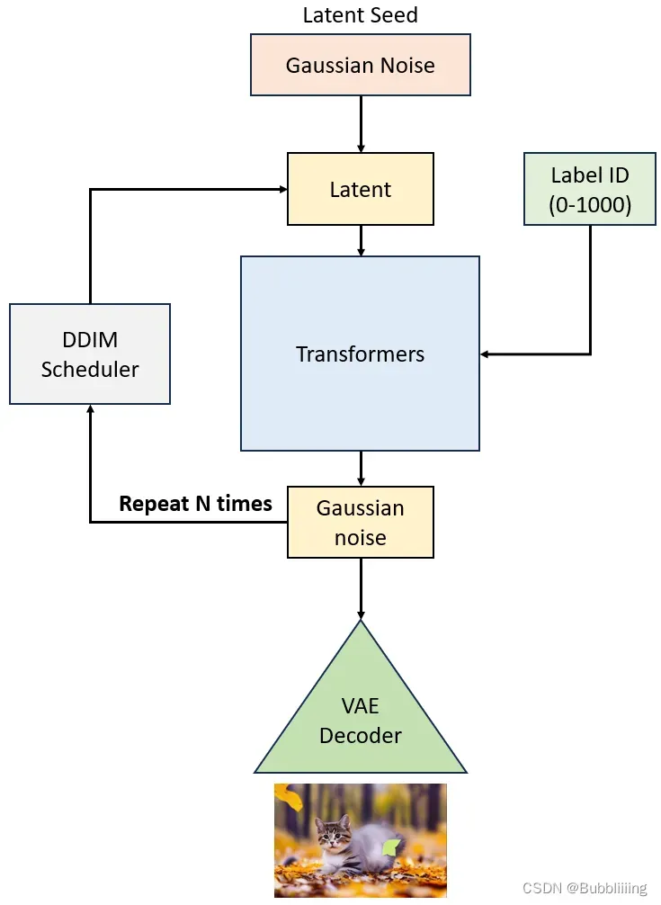
生成流程分为两个部分：
1、生成正态分布向量后进行若干次采样。
2、进行解码。

由于DiT只能按照类别进行图片生成，所以无需对文本进行编码，直接传入类别的对应的id（0-1000）即可指定类别。

# --------------------------------- #
#   前处理
# --------------------------------- #
# 生成latent
latents = randn_tensor(
    shape=(batch_size, latent_channels, latent_size, latent_size),
    generator=generator,
    device=self._execution_device,
    dtype=self.transformer.dtype,
)
latent_model_input = torch.cat([latents] * 2) if guidance_scale > 1 else latents

# 将输入的label 与 null label进行concat，null label是负向提示类。
class_labels = torch.tensor(class_labels, device=self._execution_device).reshape(-1)
class_null = torch.tensor([1000] * batch_size, device=self._execution_device)
class_labels_input = torch.cat([class_labels, class_null], 0) if guidance_scale > 1 else class_labels

# 设置生成的步数
self.scheduler.set_timesteps(num_inference_steps)

# --------------------------------- #
#   扩散生成
# --------------------------------- #
# 开始N步扩散的循环
for t in self.progress_bar(self.scheduler.timesteps):
    if guidance_scale > 1:
        half = latent_model_input[: len(latent_model_input) // 2]
        latent_model_input = torch.cat([half, half], dim=0)
    latent_model_input = self.scheduler.scale_model_input(latent_model_input, t)
    
    # 处理timesteps
    timesteps = t
    if not torch.is_tensor(timesteps):
        is_mps = latent_model_input.device.type == "mps"
        if isinstance(timesteps, float):
            dtype = torch.float32 if is_mps else torch.float64
        else:
            dtype = torch.int32 if is_mps else torch.int64
        timesteps = torch.tensor([timesteps], dtype=dtype, device=latent_model_input.device)
    elif len(timesteps.shape) == 0:
        timesteps = timesteps[None].to(latent_model_input.device)
    # broadcast to batch dimension in a way that's compatible with ONNX/Core ML
    timesteps = timesteps.expand(latent_model_input.shape[0])

    # 将隐含层特征、时间步和种类输入传入到transformers中
    noise_pred = self.transformer(
        latent_model_input, timestep=timesteps, class_labels=class_labels_input
    ).sample

    # perform guidance
    if guidance_scale > 1:
        # 在通道上做分割，取出生图部分的通道
        eps, rest = noise_pred[:, :latent_channels], noise_pred[:, latent_channels:]
        cond_eps, uncond_eps = torch.split(eps, len(eps) // 2, dim=0)

        half_eps = uncond_eps + guidance_scale * (cond_eps - uncond_eps)
        eps = torch.cat([half_eps, half_eps], dim=0)

        noise_pred = torch.cat([eps, rest], dim=1)

    # 对结果进行分割，取出生图部分的通道
    if self.transformer.config.out_channels // 2 == latent_channels:
        model_output, _ = torch.split(noise_pred, latent_channels, dim=1)
    else:
        model_output = noise_pred

    # 通过采样器将这一步噪声施加到隐含层
    latent_model_input = self.scheduler.step(model_output, t, latent_model_input).prev_sample

if guidance_scale > 1:
    latents, _ = latent_model_input.chunk(2, dim=0)
else:
    latents = latent_model_input

# --------------------------------- #
#   后处理
# --------------------------------- #
# 通过vae进行解码
latents = 1 / self.vae.config.scaling_factor * latents
samples = self.vae.decode(latents).sample

samples = (samples / 2 + 0.5).clamp(0, 1)

# 转化为float32类别
samples = samples.cpu().permute(0, 2, 3, 1).float().numpy()

1、采样流程

a、生成初始噪声

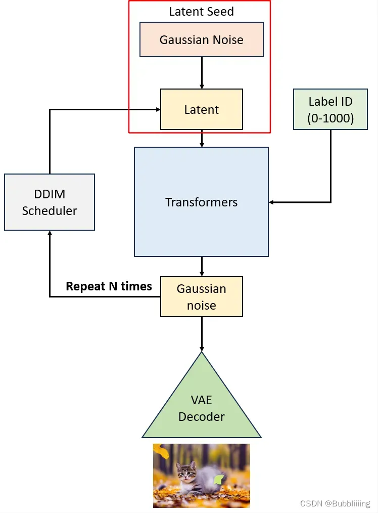
在生成初始噪声前介绍一下VAE，VAE是变分自编码器，可以将输入图片进行编码，一个高宽原本为256x256x3的图片在使用VAE编码后会变成32x32x4，这个4是人为设定的，不必纠结为什么不是3。这个时候我们就使用一个相对简单的矩阵代替原有的256x256x3的图片了，传输与存储成本就很低。在实际要去看的时候，可以对32x32x4的矩阵进行解码，获得256x256x3的图片。

因此，如果 我们要生成一个256x256x3的图片，那么我们只需要初始化一个32x32x4的隐向量，在隐空间进行扩散即可。在隐空间扩散好后，再使用解码器就可以生成256x256x3的图像。

在代码中，我们确实是这么做的，初始噪声的生成函数为randn_tensor，是diffusers自带的一个函数，尽管它写的很长，但实际生成初始噪声的代码只有一行：

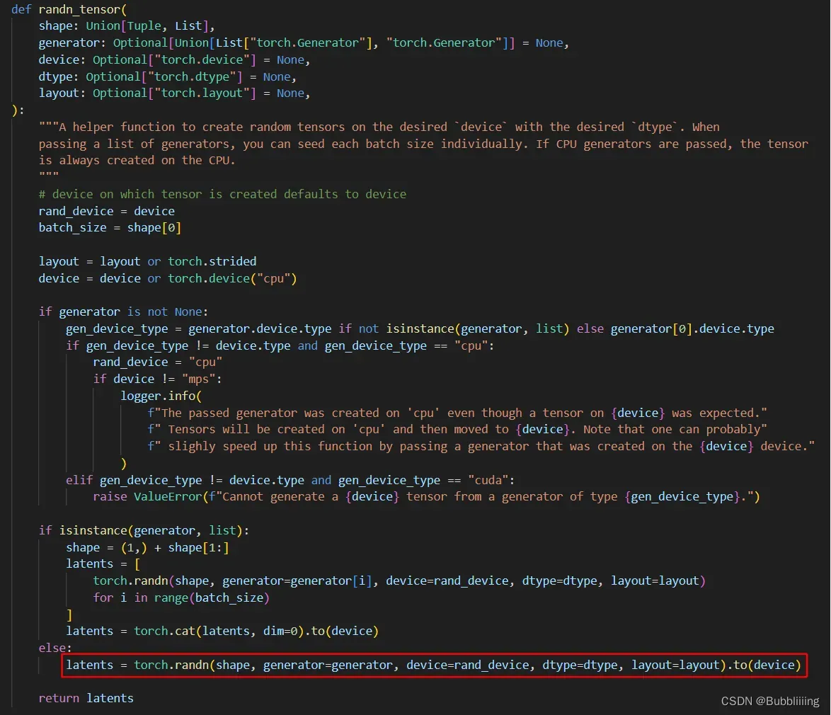
latents = torch.randn(shape, generator=generator, device=rand_device, dtype=dtype, layout=layout).to(device)

代码本来位于diffusers的工具文件中，为了方便查看，我将其复制到nets/pipeline.py中。

b、对噪声进行N次采样

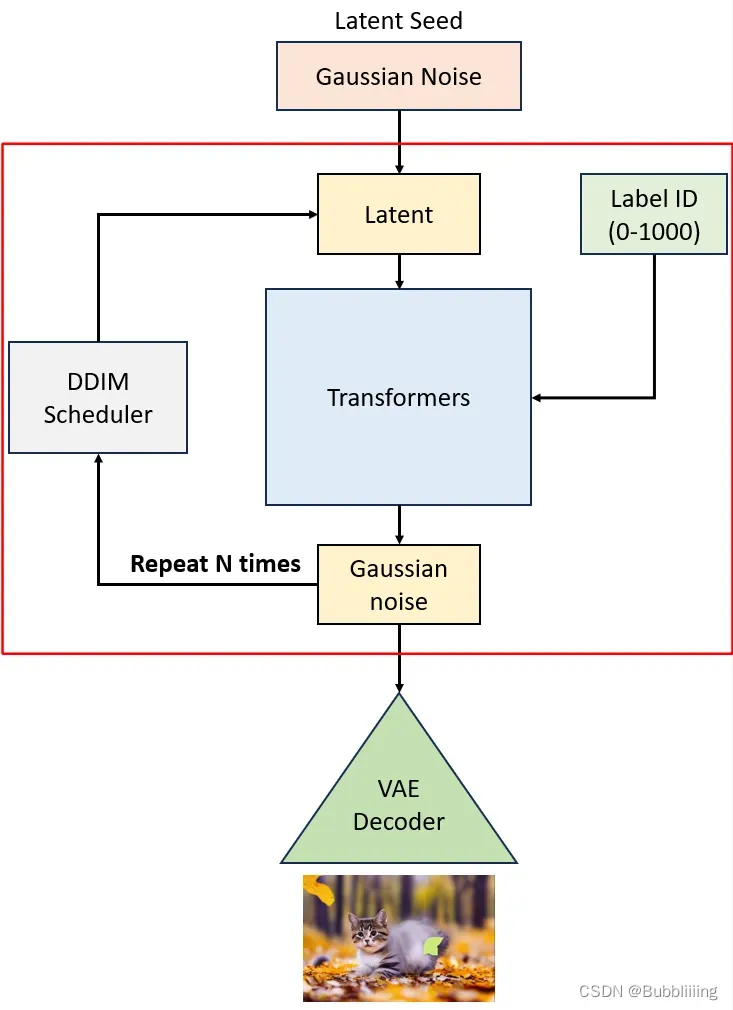
既然Stable Diffusion是一个不断扩散的过程，那么少不了不断的去噪声，那么怎么去噪声便是一个问题。

在上一步中，我们已经获得了一个latents，它是一个符合正态分布的向量，我们便从它开始去噪声。

在代码中，我们有一个对时间步的循环，会不断的将隐含层向量输入到transformers中进行噪声预测，并且一步一步的去噪。

# --------------------------------- #
#   扩散生成
# --------------------------------- #
# 开始N步扩散的循环
for t in self.progress_bar(self.scheduler.timesteps):
    if guidance_scale > 1:
        half = latent_model_input[: len(latent_model_input) // 2]
        latent_model_input = torch.cat([half, half], dim=0)
    latent_model_input = self.scheduler.scale_model_input(latent_model_input, t)
    
    # 处理timesteps
    timesteps = t
    if not torch.is_tensor(timesteps):
        is_mps = latent_model_input.device.type == "mps"
        if isinstance(timesteps, float):
            dtype = torch.float32 if is_mps else torch.float64
        else:
            dtype = torch.int32 if is_mps else torch.int64
        timesteps = torch.tensor([timesteps], dtype=dtype, device=latent_model_input.device)
    elif len(timesteps.shape) == 0:
        timesteps = timesteps[None].to(latent_model_input.device)
    # broadcast to batch dimension in a way that's compatible with ONNX/Core ML
    timesteps = timesteps.expand(latent_model_input.shape[0])

    # 将隐含层特征、时间步和种类输入传入到transformers中
    noise_pred = self.transformer(
        latent_model_input, timestep=timesteps, class_labels=class_labels_input
    ).sample

    # perform guidance
    if guidance_scale > 1:
        # 在通道上做分割，取出生图部分的通道
        eps, rest = noise_pred[:, :latent_channels], noise_pred[:, latent_channels:]
        cond_eps, uncond_eps = torch.split(eps, len(eps) // 2, dim=0)

        half_eps = uncond_eps + guidance_scale * (cond_eps - uncond_eps)
        eps = torch.cat([half_eps, half_eps], dim=0)

        noise_pred = torch.cat([eps, rest], dim=1)

    # 对结果进行分割，取出生图部分的通道
    if self.transformer.config.out_channels // 2 == latent_channels:
        model_output, _ = torch.split(noise_pred, latent_channels, dim=1)
    else:
        model_output = noise_pred

    # 通过采样器将这一步噪声施加到隐含层
    latent_model_input = self.scheduler.step(model_output, t, latent_model_input).prev_sample

c、单次采样解析

I、预测噪声

在进行单次采样前，需要首先判断是否有负向提示类，如果有，我们需要同时处理负向提示类，否则仅仅需要处理正向提示类。实际使用的时候一般都有负向提示类（效果会好一些），所以默认进入对应的处理过程。

在处理负向提示类时，我们对输入进来的隐向量进行复制，一个属于正向提示类（0-999），一个属于负向提示类（1000）。它们是在batch_size维度进行堆叠，二者不会互相影响。然后我们将正向提示类和负向提示类（1000）也在batch_size维度堆叠。代码中，如果guidance_scale＞1则代表需要负向提示类。

# --------------------------------- #
#   前处理
# --------------------------------- #
# 生成latent
latents = randn_tensor(
    shape=(batch_size, latent_channels, latent_size, latent_size),
    generator=generator,
    device=self._execution_device,
    dtype=self.transformer.dtype,
)
latent_model_input = torch.cat([latents] * 2) if guidance_scale > 1 else latents

# 将输入的label 与 null label进行concat，null label是负向提示类。
class_labels = torch.tensor(class_labels, device=self._execution_device).reshape(-1)
class_null = torch.tensor([1000] * batch_size, device=self._execution_device)
class_labels_input = torch.cat([class_labels, class_null], 0) if guidance_scale > 1 else class_labels

堆叠完后，我们将隐向量、步数和类别条件一起传入网络中，将结果在bs维度进行使用chunk进行分割。

因为我们在堆叠时，正向提示类放在了前面。因此分割好后，前半部分cond_eps属于利用正向提示类得到的，后半部分uncond_eps属于利用负向提示类得到的，我们本质上应该扩大正向提示类的影响，远离负向提示类的影响。因此，我们使用cond_eps-uncond_eps计算二者的距离，使用scale扩大二者的距离。在uncond_eps基础上，得到最后的隐向量。

# 堆叠完后，隐向量、步数和prompt条件一起传入网络中，将结果在bs维度进行使用chunk进行分割
e_t_uncond, e_t = self.model.apply_model(x_in, t_in, c_in).chunk(2)
e_t = e_t_uncond + unconditional_guidance_scale * (e_t - e_t_uncond)

此时获得的eps就是通过隐向量和提示类共同获得的预测噪声啦。

II、施加噪声

在获得噪声后，我们还要将获得的新噪声，按照一定的比例添加到原来的原始噪声上。

diffusers的代码并没有将施加噪声的代码写在明面上，而是使用采样器的step方法替代，采样流程与DDIM一致，因此直接参考DDIM公式即可，此前，在Stable Diffusion相关博文中写到过DDIM公式，可以参考对应博文了解一下。

latent_model_input = self.scheduler.step(model_output, t, latent_model_input).prev_sample

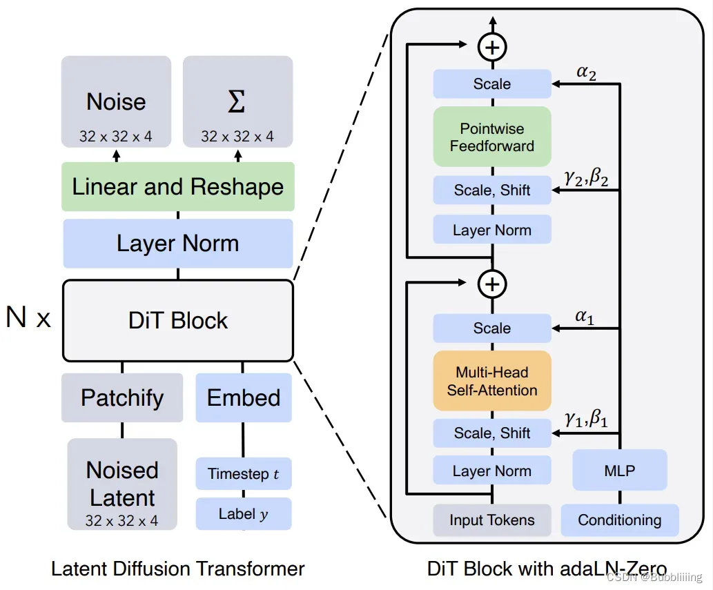
d、预测噪声过程中的网络结构解析

这个部分是DiT与Stable Diffusion最大的不同，DiT将网络结构从Unet转换成了Transformers，

i、adaLN-Zero结构解析

Transformers主要做的工作是结合 时间步t 和 类别 计算这一时刻的噪声。此处的Transformers结构与VIT中的Transformers基本一致，但为了融合时间步t和类别，新增了一个Embed层和adaLN-Zero结构。

• Embed层主要是将输入进来的timestep和label进行向量化。
• adaLN-Zero则是通过全连接对向量化后的timestep和label进行映射，然后分为6个部分，分别作用于DiT的不同阶段用于缩放（scale）、偏置（shift、bias）与门函数（gate）。

如下是Embed层和adaLN-Zero结构的代码与示意图：

class CombinedTimestepLabelEmbeddings(nn.Module):
    def __init__(self, num_classes, embedding_dim, class_dropout_prob=0.1):
        super().__init__()

        self.time_proj = Timesteps(num_channels=256, flip_sin_to_cos=True, downscale_freq_shift=1)
        self.timestep_embedder = TimestepEmbedding(in_channels=256, time_embed_dim=embedding_dim)
        self.class_embedder = LabelEmbedding(num_classes, embedding_dim, class_dropout_prob)

    def forward(self, timestep, class_labels, hidden_dtype=None):
        timesteps_proj = self.time_proj(timestep)
        timesteps_emb = self.timestep_embedder(timesteps_proj.to(dtype=hidden_dtype))  # (N, D)

        class_labels = self.class_embedder(class_labels)  # (N, D)

        conditioning = timesteps_emb + class_labels  # (N, D)

        return conditioning

class AdaLayerNormZero(nn.Module):
    """
    Norm layer adaptive layer norm zero (adaLN-Zero).
    """

    def __init__(self, embedding_dim, num_embeddings):
        super().__init__()

        self.emb = CombinedTimestepLabelEmbeddings(num_embeddings, embedding_dim)

        self.silu = nn.SiLU()
        self.linear = nn.Linear(embedding_dim, 6 * embedding_dim, bias=True)
        self.norm = nn.LayerNorm(embedding_dim, elementwise_affine=False, eps=1e-6)

    def forward(self, x, timestep, class_labels, hidden_dtype=None):
        emb = self.linear(self.silu(self.emb(timestep, class_labels, hidden_dtype=hidden_dtype)))
        shift_msa, scale_msa, gate_msa, shift_mlp, scale_mlp, gate_mlp = emb.chunk(6, dim=1)
        x = self.norm(x) * (1 + scale_msa[:, None]) + shift_msa[:, None]
        return x, gate_msa, shift_mlp, scale_mlp, gate_mlp

ii、patch分块处理

在代码中，我们使用一个PatchEmbed类对输入的隐含层向量进行分块，该操作便是VIT中的patchc操作，通过卷积进行类似于下采样的操作，可以减少计算量。

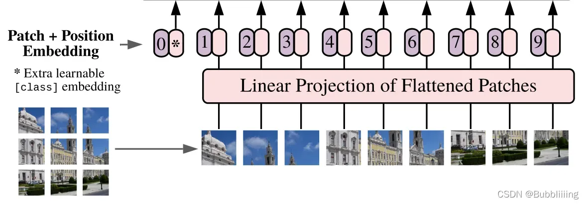
如下为patch分块处理的代码，核心是使用步长和卷积核大小一样的Conv2d模块进行处理，由于步长和卷积核大小一致，每个图片区域的特征提取过程就不会有重叠。

我们初始化生成的隐含层向量为32x32x4。在DiT-XL-2中，patch处理的步长和卷积核大小为2，通道为1152，在处理完成后，特征的通道上升，高宽被压缩，此时我们获得一个16x16x1152的新特征，然后我们将其在长宽上进行平铺，获得一个256×1152的向量，并且加上位置信息。

class PatchEmbed(nn.Module):
    """2D Image to Patch Embedding"""

    def __init__(
        self,
        height=224,
        width=224,
        patch_size=16,
        in_channels=3,
        embed_dim=768,
        layer_norm=False,
        flatten=True,
        bias=True,
    ):
        super().__init__()

        num_patches = (height // patch_size) * (width // patch_size)
        self.flatten = flatten
        self.layer_norm = layer_norm

        self.proj = nn.Conv2d(
            in_channels, embed_dim, kernel_size=(patch_size, patch_size), stride=patch_size, bias=bias
        )
        if layer_norm:
            self.norm = nn.LayerNorm(embed_dim, elementwise_affine=False, eps=1e-6)
        else:
            self.norm = None

        pos_embed = get_2d_sincos_pos_embed(embed_dim, int(num_patches**0.5))
        self.register_buffer("pos_embed", torch.from_numpy(pos_embed).float().unsqueeze(0), persistent=False)

    def forward(self, latent):
        latent = self.proj(latent)
        if self.flatten:
            latent = latent.flatten(2).transpose(1, 2)  # BCHW -> BNC
        if self.layer_norm:
            latent = self.norm(latent)
        return latent + self.pos_embed

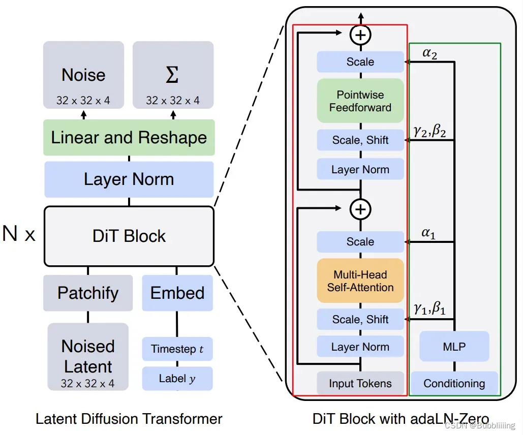
iii、Transformer特征提取

此后，我们将向量传入Transformer中进行特征提取，对应图中的DiT Block。

256×1152的特征会通过图中红框的部分，而时间步t 和 类别会通过途中绿框的部分。

红框部分的结构，除了缩放（scale）、偏置（shift、bias）与门函数（gate，对应图中的α，代码中是gate但图中写scale）外，其它部分与VIT一模一样，可参考博文VIT结构解析进行了解，主要工作的模块是Self-Attention和Pointwise Feedforward（MLP）。这两个模块的输入和输出均为256×1152的特征。

而缩放（scale）、偏置（shift、bias）与门函数（gate）分别对应了图中的γ、β和α。通过adaLN-Zero结构获得，γ、β分别在 Self-Attention和Pointwise Feedforward 的处理前 进行特征的 缩放与偏置 ，而Pointwise Feedforward则在 Self-Attention和Pointwise Feedforward 的处理后 进行特征的 缩放。在代码中我添加了中文注释，方便读者区分添加缩放、偏置和门函数的位置。

DiT Block的输入和输出特征均为256×1152。

class BasicTransformerBlock(nn.Module):
    def __init__(
        self,
        dim: int,
        num_attention_heads: int,
        attention_head_dim: int,
        dropout=0.0,
        cross_attention_dim: Optional[int] = None,
        activation_fn: str = "geglu",
        num_embeds_ada_norm: Optional[int] = None,
        attention_bias: bool = False,
        only_cross_attention: bool = False,
        double_self_attention: bool = False,
        upcast_attention: bool = False,
        norm_elementwise_affine: bool = True,
        norm_type: str = "layer_norm",
        final_dropout: bool = False,
    ):
        super().__init__()
        .......

    def forward(
        self,
        hidden_states: torch.FloatTensor,
        attention_mask: Optional[torch.FloatTensor] = None,
        encoder_hidden_states: Optional[torch.FloatTensor] = None,
        encoder_attention_mask: Optional[torch.FloatTensor] = None,
        timestep: Optional[torch.LongTensor] = None,
        cross_attention_kwargs: Dict[str, Any] = None,
        class_labels: Optional[torch.LongTensor] = None,
    ):
        # Notice that normalization is always applied before the real computation in the following blocks.
        # 1. Self-Attention
        if self.use_ada_layer_norm:
            norm_hidden_states = self.norm1(hidden_states, timestep)
        elif self.use_ada_layer_norm_zero:
            # 在norm1中，已经进行了输入特征的缩放与偏置
            norm_hidden_states, gate_msa, shift_mlp, scale_mlp, gate_mlp = self.norm1(
                hidden_states, timestep, class_labels, hidden_dtype=hidden_states.dtype
            )
        else:
            norm_hidden_states = self.norm1(hidden_states)

        cross_attention_kwargs = cross_attention_kwargs if cross_attention_kwargs is not None else {}

        attn_output = self.attn1(
            norm_hidden_states,
            encoder_hidden_states=encoder_hidden_states if self.only_cross_attention else None,
            attention_mask=attention_mask,
            **cross_attention_kwargs,
        )
        # 在self attention后，再次进行了特征的缩放（gate）
        if self.use_ada_layer_norm_zero:
            attn_output = gate_msa.unsqueeze(1) * attn_output
        hidden_states = attn_output + hidden_states

        # 2. Cross-Attention
        if self.attn2 is not None:
            norm_hidden_states = (
                self.norm2(hidden_states, timestep) if self.use_ada_layer_norm else self.norm2(hidden_states)
            )

            attn_output = self.attn2(
                norm_hidden_states,
                encoder_hidden_states=encoder_hidden_states,
                attention_mask=encoder_attention_mask,
                **cross_attention_kwargs,
            )
            hidden_states = attn_output + hidden_states

        # 3. Feed-forward
        norm_hidden_states = self.norm3(hidden_states)

        # 在mlp前，进行了输入特征的缩放与偏置
        if self.use_ada_layer_norm_zero:
            norm_hidden_states = norm_hidden_states * (1 + scale_mlp[:, None]) + shift_mlp[:, None]

        if self._chunk_size is not None:
            # "feed_forward_chunk_size" can be used to save memory
            if norm_hidden_states.shape[self._chunk_dim] % self._chunk_size != 0:
                raise ValueError(
                    f"`hidden_states` dimension to be chunked: {norm_hidden_states.shape[self._chunk_dim]} has to be divisible by chunk size: {self._chunk_size}. Make sure to set an appropriate `chunk_size` when calling `unet.enable_forward_chunking`."
                )

            num_chunks = norm_hidden_states.shape[self._chunk_dim] // self._chunk_size
            ff_output = torch.cat(
                [self.ff(hid_slice) for hid_slice in norm_hidden_states.chunk(num_chunks, dim=self._chunk_dim)],
                dim=self._chunk_dim,
            )
        else:
            ff_output = self.ff(norm_hidden_states)

        # 在mlp后，再次进行了特征的缩放（gate）
        if self.use_ada_layer_norm_zero:
            ff_output = gate_mlp.unsqueeze(1) * ff_output

        hidden_states = ff_output + hidden_states

        return hidden_states

iv、上采样

虽然这个部分学名可能不叫上采样，但是我觉得用上采样来描述它还是比较合适的，因为我们前面做过patch分块处理，所以隐含层的高宽被压缩，而这一步，则是将隐含层的高宽再还原回去。

在这里我们会对256×1152进行两次全连接+一次LayerNorm，两次全连接的神经元个数分别为2304和patch_size * patch_size * out_channels。第一次全连接目的是扩宽通道数，第二次全链接则是还原高宽。两次全连接后，在DiT-XL-2中，out_channels为8（8可拆分为4 + 4，前面的4用于直接预测噪声，后面的4用于根据均值和方差计算KL散度），特征层的shape从256×1152变为256×32。

然后我们会进行一系列shape变换，首先将256×1152变为16x16x2x2x8，然后进行转置变为8x16x2x16x2，然后还原高宽变为8x32x32。此时上采样结束。该部分对应了图中的Linear And Reshape。

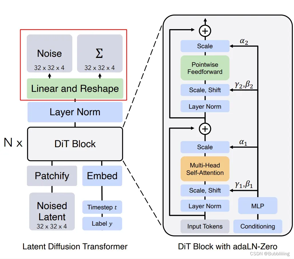
上采样代码如下所示：

# 3. Output
conditioning = self.transformer_blocks[0].norm1.emb(
    timestep, class_labels, hidden_dtype=hidden_states.dtype
)
shift, scale = self.proj_out_1(F.silu(conditioning)).chunk(2, dim=1)
hidden_states = self.norm_out(hidden_states) * (1 + scale[:, None]) + shift[:, None]
hidden_states = self.proj_out_2(hidden_states)

# unpatchify
height = width = int(hidden_states.shape[1] ** 0.5)
hidden_states = hidden_states.reshape(
    shape=(-1, height, width, self.patch_size, self.patch_size, self.out_channels)
)
hidden_states = torch.einsum("nhwpqc->nchpwq", hidden_states)
output = hidden_states.reshape(
    shape=(-1, self.out_channels, height * self.patch_size, width * self.patch_size)
)

3、隐空间解码生成图片

通过上述步骤，已经可以多次采样获得结果，然后我们便可以通过隐空间解码生成图片。

隐空间解码生成图片的过程非常简单，将上文多次采样后的结果，使用vae的decode方法即可生成图片。

# --------------------------------- #
#   后处理
# --------------------------------- #
# 通过vae进行解码
latents = 1 / self.vae.config.scaling_factor * latents
samples = self.vae.decode(latents).sample

samples = (samples / 2 + 0.5).clamp(0, 1)

# 转化为float32类别
samples = samples.cpu().permute(0, 2, 3, 1).float().numpy()

类别到图像预测过程代码

整体预测代码如下：

import torch
import json
import os
from diffusers import DPMSolverMultistepScheduler, AutoencoderKL

from nets.transformer_2d import Transformer2DModel
from nets.pipeline import DiTPipeline

# 模型路径
model_path = "model_data/DiT-XL-2-256"

# 初始化DiT的各个组件
scheduler = DPMSolverMultistepScheduler.from_pretrained(model_path, subfolder="scheduler")
transformer = Transformer2DModel.from_pretrained(model_path, subfolder="transformer")
vae = AutoencoderKL.from_pretrained(model_path, subfolder="vae")
id2label = json.load(open(os.path.join(model_path, "model_index.json"), "r"))['id2label']

# 初始化DiT的Pipeline
pipe = DiTPipeline(scheduler=scheduler, transformer=transformer, vae=vae, id2label=id2label)
pipe = pipe.to("cuda")

# imagenet种类 对应的 名称
words = ["white shark", "umbrella"]
# 获得imagenet对应的ids
class_ids = pipe.get_label_ids(words)
# 设置seed
generator = torch.manual_seed(42)

# pipeline前传
output = pipe(class_labels=class_ids, num_inference_steps=25, generator=generator)

# 保存图片
for index, image in enumerate(output.images):
    image.save(f"output-{index}.png")