GEE|用随机森林进行农作物分类的一次尝试

参考：https://www.bilibili.com/video/BV1HL4y1M7ue?spm_id_from=333.337.search-card.all.click

一、前期探索

前言：用别人已经分类好的结果来分类，小编也不知道自己在干什么呢！~_~
前期准备：把2017-2019年的分类结果按掩膜提取到自己的研究区，并用重分类提取出玉米、大豆栅格。再取交集找到这三年都种玉米或都种大豆的地块。
先上一下这部分结果：
17年玉米种植区分布：

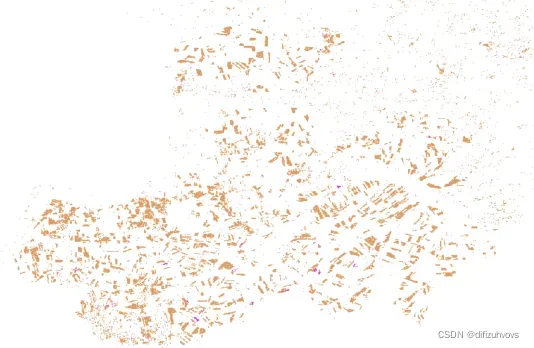
18年玉米种植区分布：

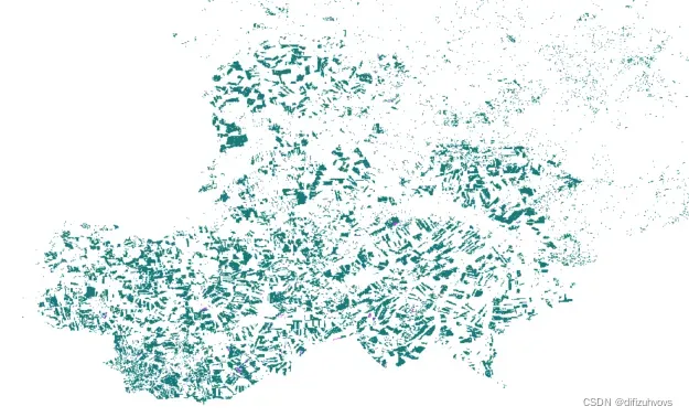
19年玉米种植区分布：

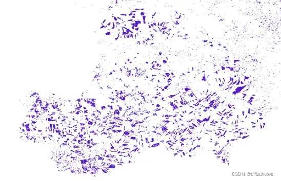
取交集后：

呃呃。。。怎么重叠部分这么少呢~_~相信大家懂得都懂，这里就看破不说破……………………………………………………

二、上传边界及样本参考

前面的步骤忽略不计。只选用2019年的分类结果，上传到GEE，10m分辨率的tif传了一下午也失败了，于是重采样到100m上传。
结果原来的4类在GEE中展示只有一类。如下图。
arcmap中的分类结果：

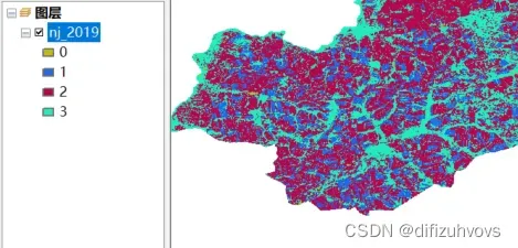
放到GEE中展示：

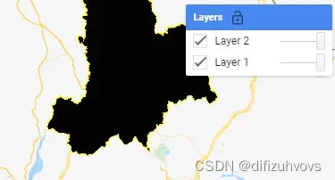
所以还是得分成“玉米”、“大豆”两类上传。
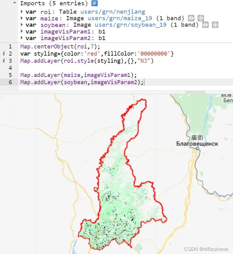
展示我们的研究区范围及分类结果。

Map.centerObject(roi,7);
var styling={color:'red',fillColor:'00000000'}
Map.addLayer(roi.style(styling),{},"NJ")

Map.addLayer(maize,imageVisParam1);
Map.addLayer(soybean,imageVisParam2);

三、建立样本数据集

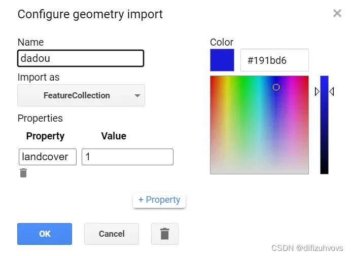
在分类结果上选取玉米种植区样本60个，大豆种植区样本60个，“其它”60个。
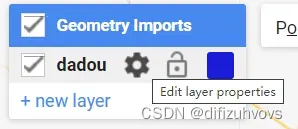
样本数据集建立方法是点击这个“添加标记”，然后点击这个设置按钮修改属性，如下三图所示。

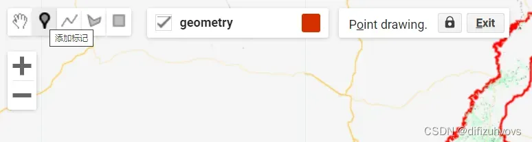
标好之后导出，免得丢失。

Export.table.toDrive({
  collection:dadou,
  description: "dadou",
  fileNamePrefix: "dadou",
  folder:'sampleShp',
  fileFormat: "SHP"
});

Export.table.toDrive({
  collection:yumi,
  description: "yumi",
  fileNamePrefix: "yumi",
  folder:'sampleShp',
  fileFormat: "SHP"
});

Export.table.toDrive({
  collection:qita,
  description: "qita",
  fileNamePrefix: "qita",
  folder:'sampleShp',
  fileFormat: "SHP"
});

四、利用随机森林分类

Map.centerObject(roi,7);
// var styling={color:'red',fillColor:'00000000'}
// Map.addLayer(roi.style(styling),{},"NJ")
// Map.addLayer(maize,imageVisParam1);
// Map.addLayer(soybean,imageVisParam2);


//选择需要裁剪的矢量数据 
var aoi = roi;


//加载矢量边框，以便于在边界内选取样本点
var empty = ee.Image().toByte();
var outline = empty.paint({
featureCollection:aoi, // 行政边界命名为fc
color:0, //颜色透明
width:3 //边界宽度
});
Map.addLayer(outline, {palette: "ff0000"}, "outline");


//Function to mask the clouds in Sentinel-2
function maskS2clouds(image) {
  var qa = image.select('QA60');

  // Bits 10 and 11 are clouds and cirrus, respectively.
  var cloudBitMask = 1 << 10;
  var cirrusBitMask = 1 << 11;

  // Both flags should be set to zero, indicating clear conditions.
  var mask = qa.bitwiseAnd(cloudBitMask).eq(0)
      .and(qa.bitwiseAnd(cirrusBitMask).eq(0));

  return image.updateMask(mask).divide(10000);
}


//Build the Sentinel 2 collection, filtered by date, bounds and percentage of cloud cover 
var dataset = ee.ImageCollection('COPERNICUS/S2_SR')
                  .filterDate('2019-01-01','2019-12-31')
                  .filterBounds(aoi)
                  .filter(ee.Filter.lt('CLOUDY_PIXEL_PERCENTAGE',10))
                  .map(maskS2clouds);
print("Sentinel 2 Image Collection",dataset);
var dem = ee.Image("NASA/NASADEM_HGT/001")


// Construct Classfication Dataset
// RS Index Cacluate(NDVI\NDWI\EVI\BSI)
var add_RS_index = function(img){
  var ndvi = img.normalizedDifference(['B8', 'B4']).rename('NDVI').copyProperties(img,['system:time_start']);
  
  var ndwi = img.normalizedDifference(['B3', 'B8']).rename('NDWI').copyProperties(img,['system:time_start']);
  
  var evi = img.expression('2.5 * ((NIR - RED) / (NIR + 6 * RED - 7.5 * BLUE + 1))', 
  {
    'NIR': img.select('B8'),
    'RED': img.select('B4'),
    'BLUE': img.select('B2')
  }).rename('EVI').copyProperties(img,['system:time_start']);
  
  var bsi = img.expression('((RED + SWIR1) - (NIR + BLUE)) / ((RED + SWIR1) + (NIR + BLUE)) ', 
  {
    'RED': img.select('B4'), 
    'BLUE': img.select('B2'),
    'NIR': img.select('B8'),
    'SWIR1': img.select('B11')
  }).rename('BSI').copyProperties(img,['system:time_start']);

  var ibi = img.expression('(2 * SWIR1 / (SWIR1 + NIR) - (NIR / (NIR + RED) + GREEN / (GREEN + SWIR1))) / (2 * SWIR1 / (SWIR1 + NIR) + (NIR / (NIR + RED) + GREEN / (GREEN + SWIR1)))', {
    'SWIR1': img.select('B11'),
    'NIR': img.select('B8'),
    'RED': img.select('B4'),
    'GREEN': img.select('B3')
  }).rename('IBI').copyProperties(img,['system:time_start']);
  
  return img.addBands([ndvi, ndwi, evi, bsi, ibi]);
};


var dataset = dataset.map(add_RS_index); 
var bands = ['B2','B3','B4','B5','B6','B7','B8','B8A','B11','NDVI','NDWI','BSI'];
var imgcol_median = dataset.select(bands).median();
var aoi_dem = dem.select('elevation').clip(aoi).rename('DEM');
var construct_img = imgcol_median.addBands(aoi_dem).clip(aoi);


//分类样本
var train_points = dadou.merge(yumi).merge(qita);

//精度评价
var withRandom = train_points.randomColumn('random');//样本点随机的排列
var split = 0.7; 
var trainingPartition = withRandom.filter(ee.Filter.lt('random', split));//筛选70%的样本作为训练样本
var testingPartition = withRandom.filter(ee.Filter.gte('random', split));//筛选30%的样本作为测试样本


var training= construct_img.sampleRegions({
  collection: trainingPartition,
  properties: ['landcover'],
  scale: 10
});

var validation= construct_img.sampleRegions({
  collection: testingPartition,
  properties: ['landcover'],
  scale: 10
});

//分类方法选择随机森林
var rf = ee.Classifier.smileRandomForest({
  numberOfTrees: 50,  
  bagFraction: 0.8
}).train({
  features: training,
  classProperty: 'landcover',
  // inputProperties: inputbands
});


//对哨兵数据进行随机森林分类
var img_classfication = construct_img.classify(rf); 


//运用测试样本分类，确定要进行函数运算的数据集以及函数
var test = validation.classify(rf);


//计算混淆矩阵
var confusionMatrix = test.errorMatrix('landcover', 'classification');
print('confusionMatrix',confusionMatrix);//面板上显示混淆矩阵
print('overall accuracy', confusionMatrix.accuracy());//面板上显示总体精度
print('kappa accuracy', confusionMatrix.kappa());//面板上显示kappa值

Map.addLayer(aoi);
Map.addLayer(img_classfication.clip(aoi), {min: 1, max: 3, palette: ['orange', 'blue', 'green']});
var class1=img_classfication.clip(aoi)


// //导出分类图
// Export.image.toDrive({  
//       image: class1,  
//       description: 'rfclass',  
//       fileNamePrefix: 'rf',  //文件命名
//       folder: "class",  //保存的文件夹
//       scale: 10,  //分辨率
//       region: aoi,  //研究区
//       maxPixels: 1e13,  //最大像元素，默认就好
//       crs: "EPSG:4326"  //设置投影
//   });

一开始用的参考视频里小姐姐的代码，但是总体分类精度和kappa系数一直显示为1，我还以为是我样本选得不够多，于是样本各增加到100，结果还是都为1，原来是代码里有些小错，改完后结果如下图。

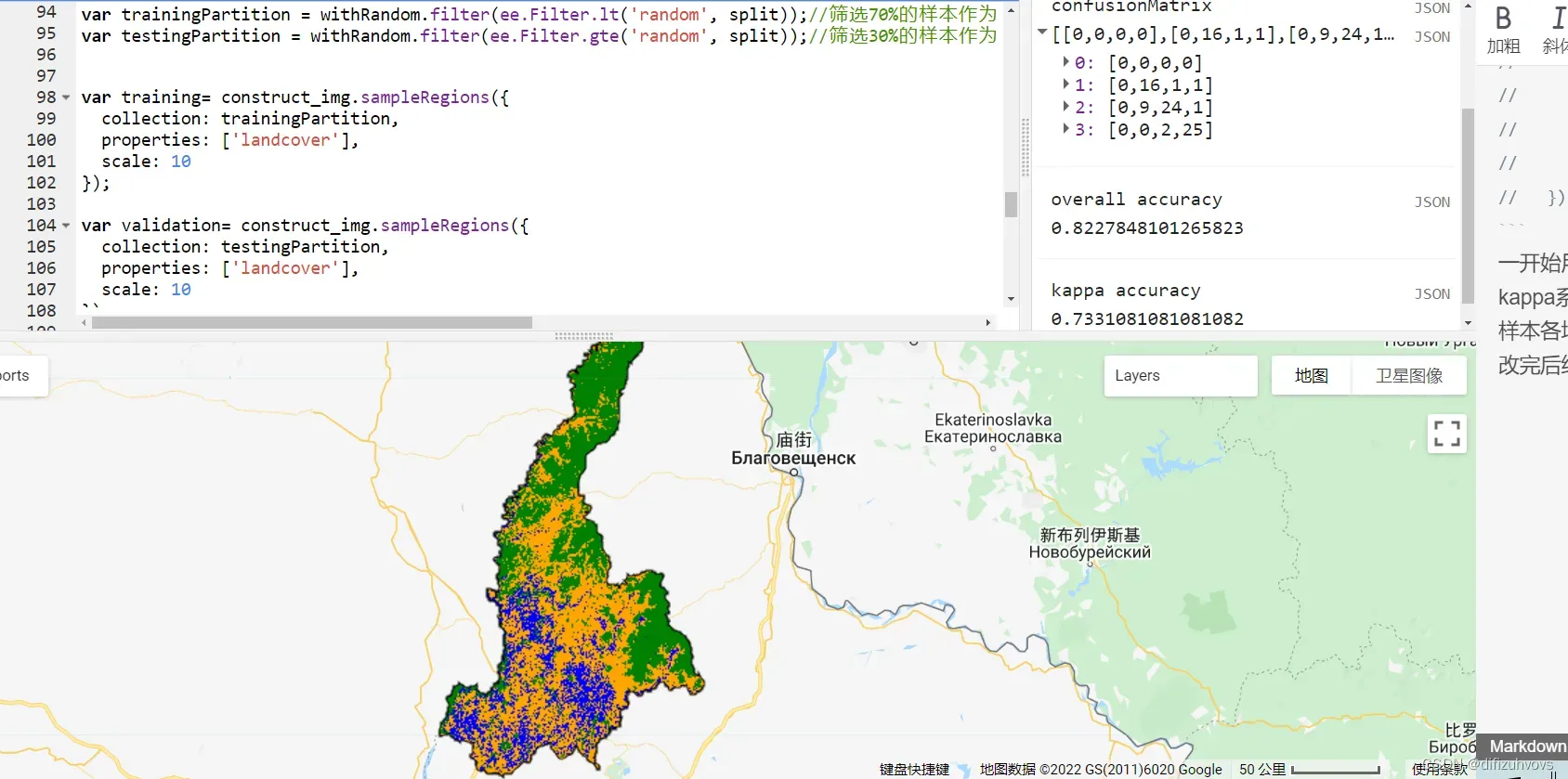
就很玄学，呵呵~

五、220511换一个试点地区

今天做就快好多了，在arcmap中进行的处理总共就这几步：

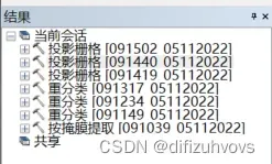
分类结果：

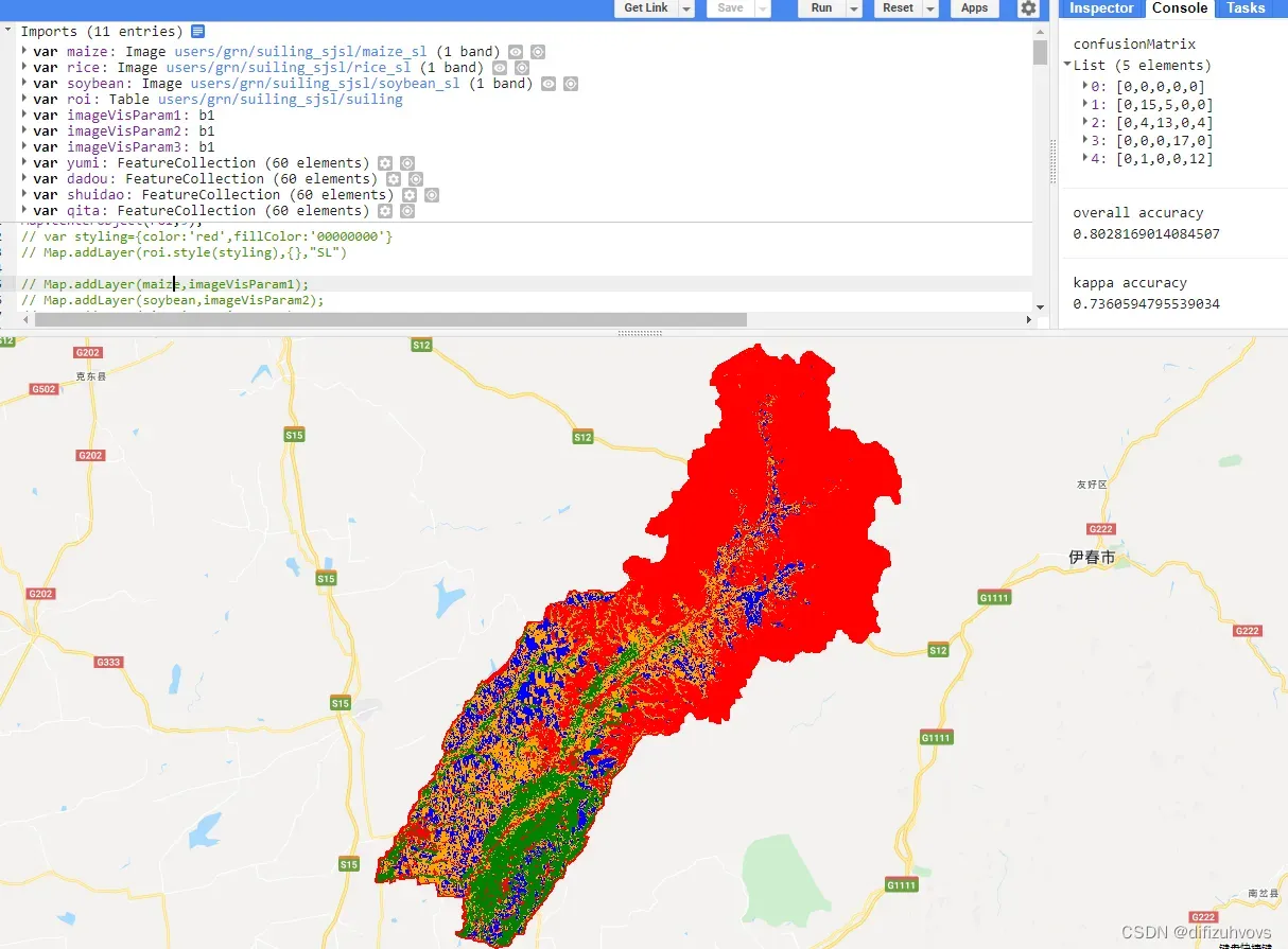
一个小时就能有个交代了=。=

文章出处登录后可见！

已经登录？立即刷新